Piecewise exponential cumulative distribution function

Computes the cumulative distribution function (CDF) or survival rate for a piecewise exponential distribution, which may be stratified.

Usage

ppwe(
  x,
  duration,
  rate,
  lower_tail = FALSE,
  stratum = NULL,
  stratum_prev = NULL
)

Arguments

x: Times at which distribution is to be computed.
duration: A numeric vector of time duration.
rate: A numeric vector of event rate.
lower_tail: Indicator of whether lower (TRUE) or upper tail (FALSE; default) of CDF is to be computed.
stratum: A vector of stratum labels parallel to duration and rate, identifying the stratum each interval belongs to, e.g., the stratum column of a data frame created by define_fail_rate(). NULL (default), or a single distinct value, means the distribution is not stratified.
stratum_prev: A numeric vector of stratum prevalences (the proportion of each stratum in the population), which must sum to 1. Either named (matched to the values of stratum) or unnamed (matched to unique(stratum) in order of appearance). Required when stratum has more than one distinct value, and ignored otherwise.

Value

A vector with cumulative distribution function or survival values.

Details

Suppose $\lambda_i$ is the failure rate in the interval $(t_{i-1},t_i], i=1,2,\ldots,M$ where $0=t_0<t_i\ldots,t_M=\infty$. The cumulative hazard function at an arbitrary time $t>0$ is then:

$$\Lambda(t)=\sum_{i=1}^M \delta(t\leq t_i)(\min(t,t_i)-t_{i-1})\lambda_i.$$ The survival at time $t$ is then $$S(t)=\exp(-\Lambda(t)).$$

For a stratified distribution, each stratum $k$ has its own intervals and failure rates, hence its own survival $S_k(t)$ as above. The marginal (population-level) survival is the mixture of those per-stratum curves, weighted by the stratum prevalences $w_k$ (summing to 1):

$$S(t)=\sum_k w_k S_k(t).$$

This is the survival of a randomly selected member of the population, and is generally not itself a piecewise exponential distribution: a mixture of exponentials is not exponential. The marginal curve can therefore not be obtained by pooling the per-stratum failure rates, and has to be averaged on the survival scale as above.

To obtain the marginal survival of the experimental arm of a design, multiply the failure rates by the hazard ratios before calling this function.

Specification

The contents of this section are shown in PDF user manual only.

Examples


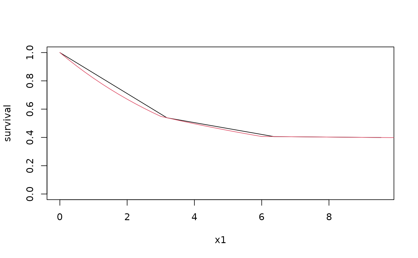
# Plot a survival function with 2 different sets of time values
# to demonstrate plot precision corresponding to input parameters.

x1 <- seq(0, 10, 10 / pi)
duration <- c(3, 3, 1)
rate <- c(.2, .1, .005)

survival <- ppwe(
  x = x1,
  duration = duration,
  rate = rate
)
plot(x1, survival, type = "l", ylim = c(0, 1))

x2 <- seq(0, 10, .25)
survival <- ppwe(
  x = x2,
  duration = duration,
  rate = rate
)
lines(x2, survival, col = 2)


# A stratified distribution: the marginal survival of the control arm of a
# design with a 30%/70% split between two biomarker strata.
fail_rate <- rbind(
  define_fail_rate(
    duration = c(6, Inf), fail_rate = log(2) / c(8, 10),
    hr = c(1, .7), dropout_rate = .001, stratum = "Biomarker positive"
  ),
  define_fail_rate(
    duration = c(6, Inf), fail_rate = log(2) / c(20, 24),
    hr = c(1, .5), dropout_rate = .001, stratum = "Biomarker negative"
  )
)
x <- seq(0, 24, 4)
stratum_prev <- c("Biomarker positive" = .3, "Biomarker negative" = .7)
with(fail_rate, ppwe(x, duration, fail_rate, stratum = stratum, stratum_prev = stratum_prev))
#> [1] 1.0000000 0.8215174 0.6919547 0.5958017 0.5151418 0.4470732 0.3893042

# The marginal curve lies between the two per-stratum curves.
split(fail_rate, ~stratum) |>
  vapply(function(d) ppwe(x, d$duration, d$fail_rate), numeric(length(x)))
#>      Biomarker negative Biomarker positive
#> [1,]          1.0000000          1.0000000
#> [2,]          0.8705506          0.7071068
#> [3,]          0.7666642          0.5176325
#> [4,]          0.6830201          0.3922920
#> [5,]          0.6085018          0.2973018
#> [6,]          0.5421134          0.2253126
#> [7,]          0.4829682          0.1707550

# The marginal survival of the experimental arm.
with(fail_rate, ppwe(x, duration, fail_rate * hr, stratum = stratum, stratum_prev = stratum_prev))
#> [1] 1.0000000 0.8215174 0.7142746 0.6547135 0.6019303 0.5549387 0.5129145