Introduction to r2rtf • r2rtf

Overview

r2rtf is an R package to create production ready tables and figures in RTF format. The R package is designed to

provide simple “verb” functions that correspond to each component of a table, to help you translate data frame to table in RTF file.
enable pipes (%>%).
only focus on table format. Data manipulation and analysis should be handled by other R packages. (e.g., tidyverse)
r2rtf minimizes package dependency

Before creating an RTF table we need to:

Figure out table layout.
Split the layout into small tasks in the form of a computer program.
Execute the program.

This document introduces r2rtf basic set of tools, and show how to transfer data frames into Table, Listing, and Figure (TLFs).

Other extended examples and features are covered in different document listed in vignettes.

Data: Adverse Events

To explore the basic RTF generation verbs in r2rtf, we will use the dataset r2rtf_adae. This dataset contain adverse events (AE) information from a clinical trial.

Below is the meaning of relevant variables. More information can be found in help page of the dataset (?r2rtf_adae)

USUBJID: Unique Subject Identifier
TRTA: Actual Treatment
AEDECOD: Dictionary-Derived Term

library(r2rtf)
library(ggplot2)
library(dplyr)
library(tidyr)

r2rtf_adae %>%
  select(USUBJID, TRTA, AEDECOD) %>%
  head(4)
##       USUBJID    TRTA                   AEDECOD
## 1 01-701-1015 Placebo APPLICATION SITE ERYTHEMA
## 2 01-701-1015 Placebo APPLICATION SITE PRURITUS
## 3 01-701-1015 Placebo                 DIARRHOEA
## 4 01-701-1023 Placebo                  ERYTHEMA

Table ready data

dplyr and tidyr packages are used for data manipulation to create a data frame that contains all the information we want to add in an RTF table.

Please note other packages can also be used for the same purpose.

In this AE example, we provide number of subjects with each type of AE by treatment group.

tbl <- r2rtf_adae %>%
  count(TRTA, AEDECOD) %>%
  pivot_wider(names_from = TRTA, values_from = n, values_fill = 0)
tbl %>% head(4)
## # A tibble: 4 × 4
##   AEDECOD        Placebo `Xanomeline High Dose` `Xanomeline Low Dose`
##   <chr>            <int>                  <int>                 <int>
## 1 ABDOMINAL PAIN       1                      2                     3
## 2 AGITATION            2                      1                     2
## 3 ALOPECIA             1                      0                     0
## 4 ANXIETY              2                      0                     4

Single table verbs

r2rtf aims to provide one function for each type of table layout. Commonly used verbs includes:

rtf_page: RTF page information
rtf_title: RTF title information
rtf_colheader: RTF column header information
rtf_body: RTF table body information
rtf_footnote: RTF footnote information
rtf_source: RTF data source information

All these verbs are designed to enables usage of pipes (%>%). A full list of all functions can be found in the package reference.

Simple Example

A minimal example below illustrates how to combine verbs using pipes to create an RTF table.

rtf_body() defines table body layout.
rtf_encode() transfers table layout information into RTF syntax.
write_rtf() saves RTF encoding into a file with file extension .rtf.

head(tbl) %>%
  rtf_body() %>% # Step 1 Add table  attributes
  rtf_encode() %>% # Step 2 Convert attributes to RTF encode
  write_rtf("rtf/intro-ae1.rtf") # Step 3 Write to a .rtf file

Column Width

If we want to adjust the width of each column to provide more space to the first column, this can be achieved by updating col_rel_width in rtf_body.

The input of col_rel_width is a vector with same length for number of columns. This argument defines the relative length of each column within a pre-defined total column width.

In this example, the defined relative width is 3:2:2:2. Only the ratio of col_rel_width is used. Therefore it is equivalent to use col_rel_width = c(6,4,4,4) or col_rel_width = c(1.5,1,1,1).

head(tbl) %>%
  rtf_body(col_rel_width = c(3, 2, 2, 2)) %>%
  # define relative width
  rtf_encode() %>%
  write_rtf("rtf/intro-ae2.rtf")

Note:

The col_rel_width in the rtf_body() function only control relative width of table body. Therefore the column header is not aligned as expected. More details will be provided in next example to take care of column header width.
The total column width is defined in the col_width argument of the rtf_page() function.

Column Headers

In the previous example, we found an issue of misaligned column header. We can fix the issue by using the rtf_colheader() function.

In rtf_colheader, colheader argument is used to provide content of column header. We used "|" to separate the columns.

head(tbl) %>%
  rtf_colheader(
    colheader = "Adverse Events | Placebo | Xanomeline High Dose | Xanomeline Low Dose",
    col_rel_width = c(3, 2, 2, 2)
  ) %>%
  rtf_body(col_rel_width = c(3, 2, 2, 2)) %>%
  rtf_encode() %>%
  write_rtf("rtf/intro-ae3.rtf")

We also allow column headers be displayed in multiple lines. If an empty column name is needed for a column, you can insert a space between two vertical lines; e.g., "name 1 | | name 3".

The col_rel_width can be used to align column header with different number of columns.

By using rtf_colheader with col_rel_width, one can customize complicated column headers. If there are multiple pages, column header will repeat at each page by default.

head(tbl, 50) %>%
  rtf_colheader(
    colheader = " | Treatment",
    col_rel_width = c(3, 6)
  ) %>%
  rtf_colheader(
    colheader = "Adverse Events | Placebo | Xanomeline High Dose | Xanomeline Low Dose",
    col_rel_width = c(3, 2, 2, 2)
  ) %>%
  rtf_body(col_rel_width = c(3, 2, 2, 2)) %>%
  rtf_encode() %>%
  write_rtf("rtf/intro-ae4.rtf")

Text Alignment

In rtf_*() functions such as rtf_body(), rtf_footnote(), the text_justification argument is used to align text. Default is "c" for center justification. To vary text justification by column, use character vector with length of vector equal to number of columns displayed (e.g., c("c","l","r")).

All possible inputs can be found in the first column of r2rtf:::justification().

r2rtf:::justification()
##   type      name rtf_code_text rtf_code_row
## 1    l      left          \\ql       \\trql
## 2    c    center          \\qc       \\trqc
## 3    r     right          \\qr       \\trqr
## 4    d   decimal          \\qj             
## 5    j justified          \\qj

Below is an example that makes the first column left-aligned and center-aligned for the rest.

head(tbl) %>%
  rtf_body(text_justification = c("l", "c", "c", "c")) %>%
  rtf_encode() %>%
  write_rtf("rtf/intro-ae5.rtf")

Text Style

In rtf_*() functions such as rtf_body(), rtf_footnote(), etc., the text_format argument is used for controlling text style. Default is NULL for normal.

All possible inputs and corresponding text style can be found in r2rtf:::font_format().

r2rtf:::font_format()
##   type        name rtf_code
## 1           normal         
## 2    b        bold      \\b
## 3    i     italics      \\i
## 4    u   underline     \\ul
## 5    s      strike \\strike
## 6    ^ superscript  \\super
## 7    _   subscript    \\sub

Combination of format type are permitted as input (e.g., "ub" for bold and underlined text). To vary text format by column, use character vector with length of vector equal to number of columns displayed (e.g., c("i", "u", "ib")).

Below is an example to make first column in bold and normal for the rest.

head(tbl) %>%
  rtf_body(text_format = c("b", "", "", "")) %>%
  rtf_encode() %>%
  write_rtf("rtf/intro-ae6.rtf")

Table Border

In rtf_*() functions such as rtf_body(), rtf_footnote(), etc., border_left, border_right, border_top, and border_bottom control the border.

In example of intro-ae4.rtf, if we want to remove the top border of "Adverse Events" in header, we can change default value "single" to "" in border_top argument as shown below.

All possible border type inputs can be found in r2rtf:::border_type(). There are 26 different border types and we only display the first six here.

head(r2rtf:::border_type())
##         name     rtf_code
## 1                        
## 2     single      \\brdrs
## 3     double     \\brdrdb
## 4        dot    \\brdrdot
## 5       dash   \\brdrdash
## 6 small dash \\brdrdashsm

head(tbl) %>%
  rtf_colheader(
    colheader = " | Treatment",
    col_rel_width = c(3, 6)
  ) %>%
  rtf_colheader(
    colheader = "Adverse Events | Placebo | Xanomeline High Dose | Xanomeline Low Dose",
    border_top = c("", "single", "single", "single"),
    col_rel_width = c(3, 2, 2, 2)
  ) %>%
  rtf_body(col_rel_width = c(3, 2, 2, 2)) %>%
  rtf_encode() %>%
  write_rtf("rtf/intro-ae7.rtf")

Title

The title(s) can be added using the rtf_title() function as showed in below example. To get guidance on how to change title text style, aligning title, and other features in the rtf_title() function, help page ?r2rtf::rtf_title() is a good resource.

We can provide a vector for the title argument. Each value is a separate line. The format can also be controlled by providing a vector input in text_format.

We used soft return to break lines in title.

head(tbl) %>%
  rtf_title(
    title = c(
      "Adverse Event Count by Treatment Group",
      "(An example)"
    ),
    text_format = c("b", "")
  ) %>%
  rtf_colheader(
    colheader = "Adverse Events | Placebo | Xanomeline High Dose | Xanomeline Low Dose",
    col_rel_width = c(3, 2, 2, 2)
  ) %>%
  rtf_body(col_rel_width = c(3, 2, 2, 2)) %>%
  rtf_encode() %>%
  write_rtf("rtf/intro-ae8.rtf")

Footnote

The footnote(s) can be added using footnote argument in the rtf_footnote() function as showed in below example.

We can provide a vector for the footnote argument. Each value is a separate line.

Below example showed the case when using as_table = TRUE (default) to display footnote inside the table body.

head(tbl) %>%
  rtf_title(title = "Adverse Event Count by Treatment Group") %>%
  rtf_colheader(
    colheader = "Adverse Events | Placebo | Xanomeline High Dose | Xanomeline Low Dose",
    col_rel_width = c(3, 2, 2, 2)
  ) %>%
  rtf_footnote(
    footnote = c(
      "Adverse events are coded according to MedDRA version 23.0",
      "adam-adae"
    ),
    as_table = TRUE
  ) %>%
  rtf_body(col_rel_width = c(3, 2, 2, 2)) %>%
  rtf_encode() %>%
  write_rtf("rtf/intro-ae9.rtf")

Below example showed the case when using as_table = FALSE to display footnote outside the table body.

head(tbl) %>%
  rtf_title(title = "Adverse Event Count by Treatment Group") %>%
  rtf_colheader(
    colheader = "Adverse Events | Placebo | Xanomeline High Dose | Xanomeline Low Dose",
    col_rel_width = c(3, 2, 2, 2)
  ) %>%
  rtf_footnote(
    footnote = c(
      "Adverse events are coded according to MedDRA version 23.0",
      "adam-adae"
    ),
    as_table = FALSE
  ) %>%
  rtf_body(col_rel_width = c(3, 2, 2, 2)) %>%
  rtf_encode() %>%
  write_rtf("rtf/intro-ae10.rtf")

Data Source

Data source can be added using source argument in the rtf_source() function as showed in below example.

Below example showed the case when using as_table = FALSE (default) to display data source outside the table body.

We can also adjust data source to be left aligned. By default the alignment matches the table border.

head(tbl) %>%
  rtf_page(col_width = 5) %>%
  # set total column width
  rtf_title(title = "Adverse Event Count by Treatment Group") %>%
  rtf_colheader(
    colheader = "Adverse Events | Placebo | Xanomeline High Dose | Xanomeline Low Dose",
    col_rel_width = c(3, 2, 2, 2)
  ) %>%
  rtf_source(
    source = "[datasource: adam-adae]",
    text_justification = "l",
    as_table = FALSE
  ) %>%
  rtf_body(col_rel_width = c(3, 2, 2, 2)) %>%
  rtf_encode() %>%
  write_rtf("rtf/intro-ae11.rtf")

Below example showed the case when using as_table = TRUE to display data source inside the table body.

head(tbl) %>%
  rtf_title(title = "Adverse Event Count by Treatment Group") %>%
  rtf_colheader(
    colheader = "Adverse Events | Placebo | Xanomeline High Dose | Xanomeline Low Dose",
    col_rel_width = c(3, 2, 2, 2)
  ) %>%
  rtf_source(
    source = "[datasource: adam-adae]",
    as_table = TRUE
  ) %>%
  rtf_body(col_rel_width = c(3, 2, 2, 2)) %>%
  rtf_encode() %>%
  write_rtf("rtf/intro-ae12.rtf")

Special Character

In the r2rtf package, '^' is a character to be converted to rtf code '\\super' to generate superscript; '_' is for subscript.

Similarly, '<=' is a r2rtf package specified character to be converted to LaTeX command '\\leq' to generate special character \(\leq\).

LaTeX commands can be used for Greek letters and math symbol such as \(\alpha\), \(\pm\), \(\infty\). You will need to use double backslash \\ to escape backslash in R. i.e. "\\alpha", "\\pm" and "\\infty". A list of LaTex commands can be found here.

Example below demonstrates this idea.

head(tbl) %>%
  rtf_title(title = "Adverse Event Count by Treatment Group{^a}") %>%
  rtf_colheader(
    colheader = "Adverse Events{\\super 1} | Placebo | Xanomeline High Dose | Xanomeline Low Dose",
    col_rel_width = c(3, 2, 2, 2)
  ) %>%
  rtf_footnote(
    footnote = c(
      "{\\super 1}Adverse events are coded according to MedDRA 20.0{<=}version {\\leq}23.0",
      "\\alpha + \\gamma <= \\infty",
      "{^a}adam-adae"
    ),
    as_table = FALSE
  ) %>%
  rtf_body(col_rel_width = c(3, 2, 2, 2)) %>%
  rtf_encode() %>%
  write_rtf("rtf/intro-ae13.rtf")

Table Color

Each cell’s text and background color are adjustable. Take intro-ae13.rtf as an example. If we want to add gray background color to cells with 0 AE, we need to create a color name matrix corresponding to each cell in table body.

Then we need to assign this background color matrix to text_background_color argument in the rtf_body() function as shown below.

Note:

When creating a color name matrix, each element needs to be a color name defined in grDevices::colours().

tbl1 <- head(tbl)
color_matrix <- ifelse(trimws(apply(tbl1, 2, as.character)) == "0", "gray", "white")
color_matrix
##      AEDECOD Placebo Xanomeline High Dose Xanomeline Low Dose
## [1,] "white" "white" "white"              "white"            
## [2,] "white" "white" "white"              "white"            
## [3,] "white" "white" "gray"               "gray"             
## [4,] "white" "white" "gray"               "white"            
## [5,] "white" "white" "white"              "white"            
## [6,] "white" "white" "white"              "white"

tbl1 %>%
  rtf_title(title = "Adverse Event Count by Treatment Group") %>%
  rtf_colheader(
    colheader = "Adverse Events | Placebo | Xanomeline High Dose | Xanomeline Low Dose",
    col_rel_width = c(3, 2, 2, 2)
  ) %>%
  rtf_body(
    col_rel_width = c(3, 2, 2, 2),
    text_background_color = color_matrix
  ) %>%
  rtf_encode() %>%
  write_rtf("rtf/intro-ae14.rtf")

Page setup

The total number of rows in each page can be controlled in nrow argument of rtf_page() function. Every lines is counted including title, subline, header, body, footnote, source, and extra rows.

The value in nrow is the maximum number of rows allowed in one page, the actual rows display can be slightly smaller.

tbl[1:50, ] %>%
  rtf_page(nrow = 40) %>%
  rtf_title(title = "Adverse Events Example") %>%
  rtf_colheader(
    colheader = "Adverse Events | Placebo | Xanomeline High Dose | Xanomeline Low Dose",
    col_rel_width = c(3, 1, 1, 1)
  ) %>%
  rtf_body(
    col_rel_width = c(3, 1, 1, 1),
    text_justification = c("l", "c", "c", "c")
  ) %>%
  rtf_encode() %>%
  write_rtf("rtf/intro-ae15.rtf")

subline_by feature

Users can use the subline_by argument in the rtf_body() function to group table by assigning the subline_by variable.

A subject line will be displayed at the beginning of each page based on the variable provided to subline_by. Different values of subline_by will be broken into different pages.

Below example shows using treatment group as the subline_by variable.

aegt5 <- r2rtf_adae %>%
  group_by(TRTA, AEDECOD) %>%
  summarise(Count = n_distinct(USUBJID)) %>%
  filter(Count > 7) %>%
  ungroup() %>%
  arrange(TRTA, desc(Count))

head(aegt5)
## # A tibble: 6 × 3
##   TRTA                 AEDECOD                   Count
##   <chr>                <chr>                     <int>
## 1 Placebo              DIARRHOEA                     9
## 2 Placebo              ERYTHEMA                      9
## 3 Placebo              PRURITUS                      8
## 4 Xanomeline High Dose PRURITUS                     26
## 5 Xanomeline High Dose APPLICATION SITE PRURITUS    22
## 6 Xanomeline High Dose APPLICATION SITE ERYTHEMA    15

aegt5 %>%
  rtf_title(title = "Top Adverse Events by Treatment Group") %>%
  rtf_colheader(colheader = "Adverse Events|Count") %>%
  rtf_body(subline_by = "TRTA") %>%
  rtf_encode() %>%
  write_rtf("rtf/intro-ae16.rtf")

page_by feature

Users can use page_by argument in the rtf_body() function to group/separate table by single cell row with assigned page_by variable’s value in it.

A row header will be generated at the beginning of each page_by group.

If new_page = TRUE, different values of group_by will be broken into different pages. Default is FALSE.

Below example showed using treatment group as page_by variable.

aegt5 %>%
  rtf_title(title = "Top Adverse Events by Treatment Group") %>%
  rtf_colheader(colheader = "Adverse Events|Count") %>%
  rtf_body(
    page_by = "TRTA",
    new_page = TRUE
  ) %>%
  rtf_encode() %>%
  write_rtf("rtf/intro-ae17.rtf")

group_by feature

Users can use the group_by argument in the rtf_body() function to display once for group variable.

Below example shows using treatment group as group_by variable.

aegt5 %>%
  rtf_title(title = "Top Adverse Events by Treatment Group") %>%
  rtf_colheader(colheader = "Treatment|Adverse Events|Count") %>%
  rtf_body(
    group_by = "TRTA",
    text_justification = c("l", "l", "c")
  ) %>%
  rtf_encode() %>%
  write_rtf("rtf/intro-ae18.rtf")

Figure

The last example showed how to insert a figure into a RTF document.

The workflow can be summarized as:

Save figures into PNG format. (e.g. using png() or ggplot2::ggsave()).
Read PNG files into R as binary file using rtf_read_figure().
Add optional features using rtf_title(), rtf_footnote(), rtf_source().
Set up page and figure options using rtf_figure().
Convert to rtf encoding using rtf_encode(doc_type = "figure"). (Note: it is important to set doc_type = "figure" as the default is doc_type = "table to set up tables).
Write rtf to a file using write_rtf().

pruritus <- r2rtf_adae %>%
  filter(AEDECOD == "PRURITUS") %>%
  group_by(TRTA, AEDECOD) %>%
  summarise(Count = n_distinct(USUBJID))

fig <- ggplot(data = pruritus, aes(x = TRTA, y = Count)) +
  xlab("") +
  geom_bar(stat = "identity")

fig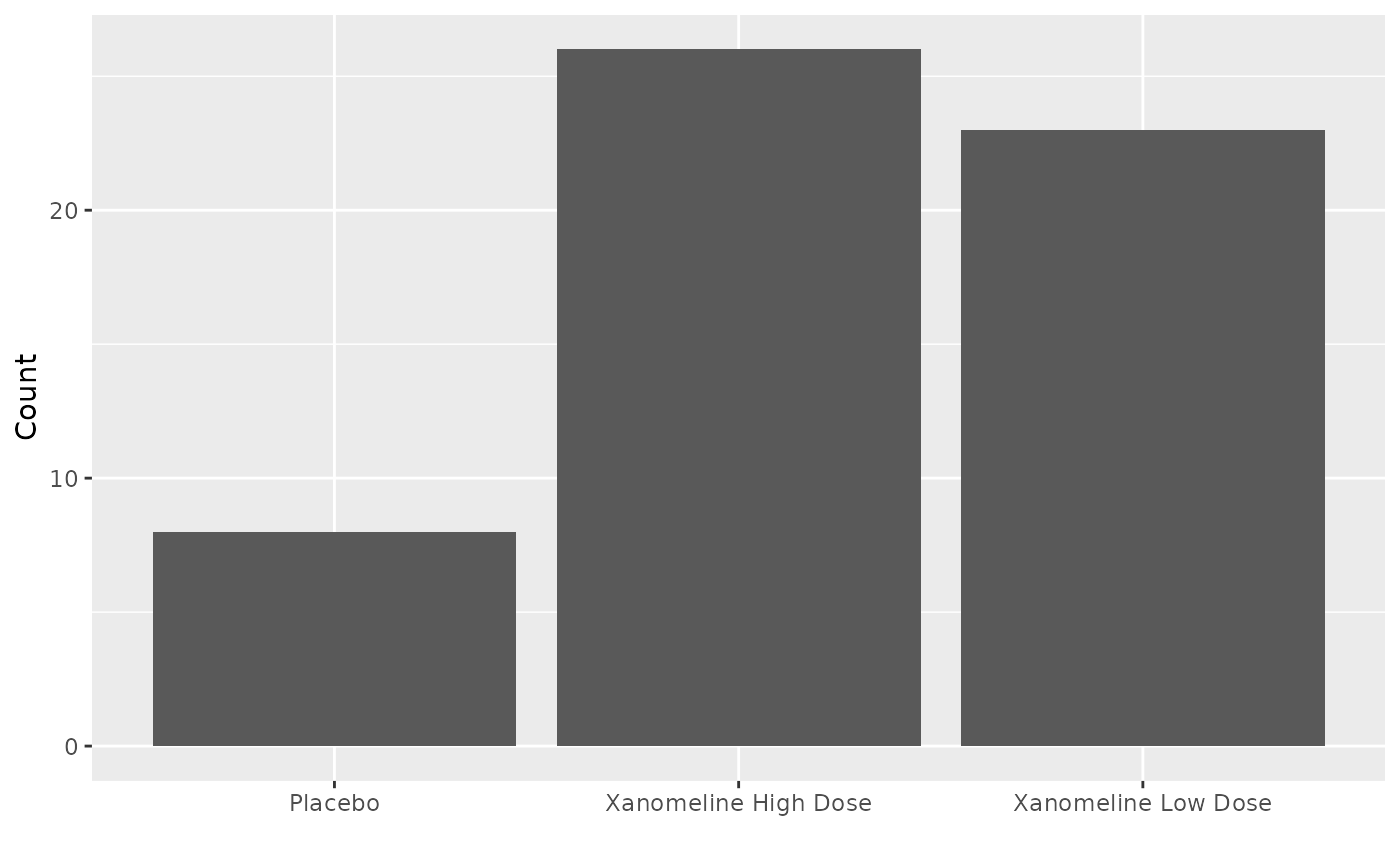

filename <- "fig/intro-fig1.png"
ggsave(filename, fig)
## Saving 7.29 x 4.51 in image

filename %>%
  rtf_read_figure() %>%
  rtf_title("Pruritus Frequency by Treatment Group") %>%
  rtf_footnote("footnote here") %>%
  rtf_source("[datasource: adam-adae]") %>%
  rtf_figure() %>%
  rtf_encode(doc_type = "figure") %>%
  write_rtf("rtf/intro-ae19.rtf")