Approximating an arbitrary hazard function

library(simtrial)
library(ggplot2)
library(dplyr)
library(survival)

This vignette uses the bshazard package. If it is not on CRAN, you can install it with

remotes::install_github("cran/bshazard")

We simulate a log-logistic distribution as an example of how to simulate a trial with an arbitrary distribution. We begin by showing hazard rates that can be used to approximate this distribution.

set.seed(123)

dloglogis <- function(x, alpha = 1, beta = 4) {
  1 / (1 + (x / alpha)^beta)
}
times <- (1:150) / 50
xx <- data.frame(
  Times = times,
  Survival = dloglogis(times, alpha = .5, beta = 4)
) |>
  mutate(
    duration = Times - lag(Times, default = 0),
    H = -log(Survival),
    rate = (H - lag(H, default = 0)) / duration / 3
  ) |>
  select(duration, rate)
ggplot(
  data = xx |> mutate(Time = lag(cumsum(duration), default = 0)),
  aes(x = Time, y = rate)
) +
  geom_line()

We assume the time scale above is in years and that enrollment occurs over the first half year at an even rate of 500 per year. We assume that observations are censored at an exponential rate of about 5% per year.

tx <- "Log-logistic"
enroll_rate <- data.frame(duration = .5, rate = 500)
dropout_rate <- data.frame(
  treatment = tx,
  duration = 3,
  rate = .05,
  period = 1,
  stratum = "All"
)
block <- rep(tx, 2)
x <- sim_pw_surv(
  n = 250, # Sample size
  block = block,
  enroll_rate = enroll_rate,
  fail_rate = xx |> mutate(
    stratum = "All",
    treatment = tx,
    period = seq_len(n()),
    stratum = "All"
  ),
  dropout_rate = dropout_rate
)

We assume the entire study lasts 3 years

y <- x |> cut_data_by_date(3)
head(y)
#>         tte event stratum    treatment
#> 1 0.5901582     1     All Log-logistic
#> 2 0.6031899     1     All Log-logistic
#> 3 1.0917184     1     All Log-logistic
#> 4 0.7423789     1     All Log-logistic
#> 5 2.2160148     1     All Log-logistic
#> 6 0.5081774     1     All Log-logistic

Now we estimate a Kaplan-Meier curve.

fit <- survfit(Surv(tte, event) ~ 1, data = y)
plot(fit, mark = "|")

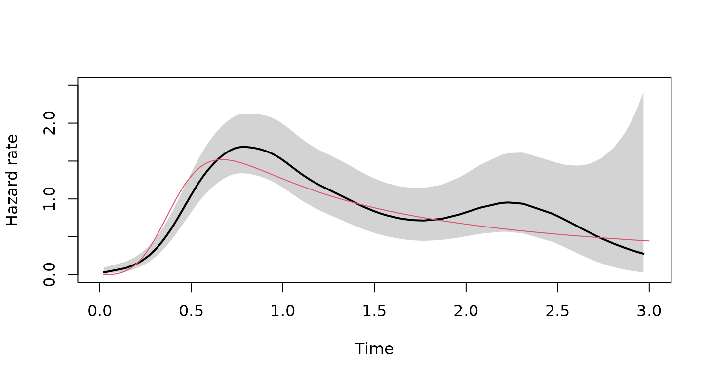
Finally, we plot the estimated hazard rate and its confidence interval as a function of time. We overlay the actual rates in red.

fit <- bshazard::bshazard(Surv(tte, event) ~ 1, data = y, nk = 120)

plot(fit, conf.int = TRUE, xlab = "Time", xlim = c(0, 3), ylim = c(0, 2.5), lwd = 2)
lines(x = times, y = (xx |> mutate(Time = lag(cumsum(duration), default = 0)))$rate, col = 2)

Keaven Anderson