Futility bounds at design and analysis under non-proportional hazards

library(gsDesign2)
library(gt)
library(dplyr)
library(tibble)
library(ggplot2)

Overview

This vignette demonstrates possible ways to set up futility bounds in clinical trial designs under the assumption of non-proportional hazards. We review the methods proposed by Wieand, Schroeder, and O’Fallon (1994) and Korn and Freidlin (2018). To be more consistent with common practice, we propose a futility bound based on \(\beta\)-spending that automatically accounts for non-proportional hazards as assumed in the design.

We start by specifying the enrollment and failure rate assumptions, following the example used by Korn and Freidlin (2018) (based on Chen (2013)).

# Enrollment assumed to be 680 patients over 12 months with no ramp-up
enroll_rate <- define_enroll_rate(duration = 12, rate = 680 / 12)

# Failure rates
## Control exponential with median of 12 mos
## Delayed effect with HR = 1 for 3 months and HR = .693 thereafter
## Censoring rate is 0
fail_rate <- define_fail_rate(
  duration = c(3, 100),
  fail_rate = -log(.5) / 12,
  hr = c(1, .693),
  dropout_rate = 0
)

## Study duration was 34.8 in Korn & Freidlin Table 1
## We change to 34.86 here to obtain 512 expected events they presented
study_duration <- 34.86

# randomization ratio (exp:control)
ratio <- 1

In this example, with 680 subjects enrolled over 12 months, we expect 512 events to occur within 34.86 months, yielding approximately 90.45% power if no interim analyses are performed.

fixedevents <- fixed_design_ahr(
  alpha = 0.025, power = NULL, ratio = ratio,
  enroll_rate = enroll_rate,
  fail_rate = fail_rate,
  study_duration = study_duration
)

fixedevents |>
  summary() |>
  select(-Bound) |>
  as_gt(footnote = "Power based on 512 events") |>
  fmt_number(columns = 3:4, decimals = 2) |>
  fmt_number(columns = 5:6, decimals = 3)

Design	N	Events	Time	AHR	alpha	Power
Fixed Design under AHR Method¹
Average hazard ratio	680	511.99	34.86	0.749	0.025	0.9045483
¹ Power based on 512 events

Beta-spending futility bound with AHR

Beta-spending allocates the Type II error rate (\(\beta\)) across interim analyses in a group sequential design. At each interim analysis, a portion of the total allowed \(\beta\) is spent to determine the futility boundary. The cumulative \(\beta\) spent up to each analysis is specified by a beta-spending function (\(\beta(t)\) with \(\beta(0) = 0\) and \(\beta(1) = \beta\)). The AHR model for the NPH alternate hypothesis accounts for the assumed early lack of benefit.

Methodology, the futility bound of IA1 (denoted as \(a_1\)) is \[ a_1 = \left\{ a_1 : \text{Pr} \left( \underbrace{Z_1 \leq a_1}_{\text{fail at IA1}} \; | \; H_1 \right) = \beta(t_1) \right\}. \] The futility bound at IA2 (denoted as \(a_2\)) is \[ a_2 = \left\{ a_2 : \text{Pr} \left( \underbrace{Z_2 \leq a_2}_{\text{fail at IA2}} \; \text{ and } \underbrace{a_1 < Z_i < b_1}_{\text{continue at IA1}} \; | \; H_1 \right) = \beta(t_2) - \beta(t_1) \right\}. \] The futility bound after IA2 can be derived in the similar logic.

In this example, the group sequential design with the \(\beta\)-spending of AHR can be derived as below.

betaspending <- gs_power_ahr(
  enroll_rate = enroll_rate,
  fail_rate = fail_rate,
  ratio = ratio,
  # 2 IAs + 1 FA
  event = 512 * c(.5, .75, 1),
  # efficacy bound
  upper = gs_b,
  upar = c(rep(Inf, 2), qnorm(.975)),
  # futility bound
  lower = gs_spending_bound,
  lpar = list(sf = gsDesign::sfLDOF, total_spend = 0.025, param = NULL, timing = NULL),
  test_lower = c(TRUE, TRUE, FALSE)
)

betaspending |>
  summary() |>
  as_gt(
    title = "Group sequential design with futility only",
    subtitle = "Beta-spending futility bound"
  )

Bound	Z	Nominal p¹	~HR at bound²	Cumulative boundary crossing probability
Group sequential design with futility only
Beta-spending futility bound
Bound	Z	Nominal p¹	~HR at bound²	Alternate hypothesis	Null hypothesis
Analysis: 1 Time: 15.4 N: 680 Events: 256 AHR: 0.81 Information fraction: 0.5
Futility	-1.29	0.9015	1.1750	0.0015	0.0985
Analysis: 2 Time: 22.9 N: 680 Events: 384 AHR: 0.77 Information fraction: 0.75
Futility	0.20	0.4206	0.9797	0.0095	0.5799
Analysis: 3 Time: 34.9 N: 680 Events: 512 AHR: 0.75 Information fraction: 1
Efficacy	1.96	0.0250	0.8409	0.9031	0.0250
¹ One-sided p-value for experimental vs control treatment. Value < 0.5 favors experimental, > 0.5 favors control.
² Approximate hazard ratio to cross bound.

Modified Wieand futility bound

The Wieand, Schroeder, and O’Fallon (1994) rule recommends stopping the trial if the observed HR exceeds 1 after 50% of planned events. Korn and Freidlin (2018) extends this approach by adding a second interim analysis at 75% of planned events, also stopping if HR > 1.

Here, we implement these futility rules by setting a Z-bound at 0, corresponding to a nominal p-value bound of approximately 0.5 at interim analyses. Fixed bounds are specified via the gs_b() function for both efficacy and futility boundaries.

The final efficacy bound is for a 1-sided nominal p-value of 0.025; the futility bound lowers this to 0.0247 as noted in the lower-right-hand corner of the table below. It is < 0.025 since the probability is computed with the binding assumption. This is an arbitrary convention; if the futility bound is ignored, this computation yields 0.025.

The design has 88.44% power. This closely matches the 88.4% power from Korn and Freidlin (2018) with 100,000 simulations which estimate the standard error for the power calculation to be 0.1%.

wieand <- gs_power_ahr(
  enroll_rate = enroll_rate, fail_rate = fail_rate,
  ratio = ratio,
  # 2 IAs + 1 FA
  event = 512 * c(.5, .75, 1),
  # efficacy bound
  upper = gs_b, upar = c(rep(Inf, 2), qnorm(.975)),
  # futility bound
  lower = gs_b, lpar = c(0, 0, -Inf),
  
)

wieand |>
  summary() |>
  as_gt(
    title = "Group sequential design with futility only at interim analyses",
    subtitle = "Wieand futility rule stops if HR > 1"
  )

Bound	Z	Nominal p¹	~HR at bound²	Cumulative boundary crossing probability
Group sequential design with futility only at interim analyses
Wieand futility rule stops if HR > 1
Bound	Z	Nominal p¹	~HR at bound²	Alternate hypothesis	Null hypothesis
Analysis: 1 Time: 15.4 N: 680 Events: 256 AHR: 0.81 Information fraction: 0.5
Futility	0.00	0.500	1.0000	0.0462	0.5000
Analysis: 2 Time: 22.9 N: 680 Events: 384 AHR: 0.77 Information fraction: 0.75
Futility	0.00	0.500	1.0000	0.0469	0.5980
Analysis: 3 Time: 34.9 N: 680 Events: 512 AHR: 0.75 Information fraction: 1
Efficacy	1.96	0.025	0.8409	0.8844	³ 0.0247
¹ One-sided p-value for experimental vs control treatment. Value < 0.5 favors experimental, > 0.5 favors control.
² Approximate hazard ratio to cross bound.
³ Cumulative alpha for final analysis (0.0247) is less than the full alpha (0.025) when the futility bound is non-binding. The smaller value subtracts the probability of crossing a futility bound before crossing an efficacy bound at a later analysis (0.025 - 0.0003 = 0.0247) under the null hypothesis.

Korn and Freidlin futility bound

Korn and Freidlin (2018) addressed scenarios with delayed treatment effects by modifying the futility rule proposed by Wieand, Schroeder, and O’Fallon (1994). Their approach sets the futility bound when at least 50% of expected events have occurred, and at least two-thirds of these events happened after 3 months from randomization.

To illustrate this, we analyze the accumulation of events over time by gsDesign2::expected_event() , distinguishing between + events occurring during the initial 3-month no-effect period and + event accumulation through the 34.86 months planned trial duration.

find_ia_time <- function(t) {
  
  e_event0 <- expected_event(
    enroll_rate = betaspending$enroll_rate |> mutate(rate = rate / (1 + ratio)), 
    fail_rate = betaspending$fail_rate |> select(stratum, fail_rate, duration, dropout_rate),
    total_duration = t, simple = FALSE)
  
  e_event1 <- expected_event(
    enroll_rate = betaspending$enroll_rate |> mutate(rate = rate / (1 + ratio) * ratio), 
    fail_rate = betaspending$fail_rate |> 
      mutate(fail_rate = fail_rate * hr) |>
      select(stratum, fail_rate, duration, dropout_rate), 
    total_duration = t, simple = FALSE)
  
  total_event <- sum(e_event0$event) + sum(e_event1$event)
  first3m_event <- sum(e_event0$event[1]) + sum(e_event1$event[1])
    
  return(2 / 3 * total_event - (total_event - first3m_event))
} 

ia1_time <- uniroot(find_ia_time, interval = c(1, 50))$root

# expected total events
e_event_overtime <- sapply(1:betaspending$analysis$time[3], function(t){
  e_event0 <- expected_event(
    enroll_rate = betaspending$enroll_rate |> mutate(rate = rate / (1 + ratio)), 
    fail_rate = betaspending$fail_rate |> select(stratum, fail_rate, duration, dropout_rate),
    total_duration = t, simple = TRUE)
  
  e_event1 <- expected_event(
    enroll_rate = betaspending$enroll_rate |> mutate(rate = rate / (1 + ratio) * ratio), 
    fail_rate = betaspending$fail_rate |> 
      mutate(fail_rate = fail_rate * hr) |>
      select(stratum, fail_rate, duration, dropout_rate), 
    total_duration = t, simple = TRUE)
  
  sum(e_event0) + sum(e_event1)
}) |> unlist()


# visualization of expected total events
p1 <- ggplot(data = data.frame(time = 1:betaspending$analysis$time[3],
                               event = e_event_overtime), 
             aes(x = time, y = event)) +
  geom_line(linewidth = 1.2) +
  geom_vline(xintercept = ia1_time, linetype = "dashed", 
             color = "red", linewidth = 1.2) +
  scale_x_continuous(breaks = c(0, 6, 12, 18, 24, 30, 36),
                     labels = c("0", "6", "12", "18", "24", "30", "36")) +
  labs(x = "Months", y =  "Events") +
  ggtitle("Expected events since study starts") +
  theme(axis.title.x = element_text(size = 18),
        axis.title.y = element_text(size = 18),
        axis.text.x = element_text(size = 20),
        axis.text.y = element_text(size = 18),
        plot.title = element_text(size = 20))

# expected events occur first 3 months
e_event_first3m <- sapply(1:betaspending$analysis$time[3], function(t){
  expected_event(enroll_rate = betaspending$enroll_rate |> mutate(rate = rate / (1 + ratio)), 
                 fail_rate = betaspending$fail_rate |> select(stratum, fail_rate, duration, dropout_rate), 
                 total_duration = t, simple = FALSE)$event[1] +
  expected_event(enroll_rate = betaspending$enroll_rate |> mutate(rate = rate / (1 + ratio) * ratio), 
                 fail_rate = betaspending$fail_rate |> 
                   mutate(fail_rate = fail_rate * hr) |>
                   select(stratum, fail_rate, duration, dropout_rate), 
                 total_duration = t, simple = FALSE)$event[1]
})

# visualization of expected events occur first 3 months
p2 <- ggplot(data = data.frame(time = 1:betaspending$analysis$time[3],
                               prop = (e_event_overtime - e_event_first3m) / e_event_overtime * 100), 
             aes(x = time, y = prop)) +
  geom_line(linewidth = 1.2) +
  scale_x_continuous(breaks = c(6, 12, 18, 24, 30, 36),
                     labels = c("6", "12", "18", "24", "30", "36")) +
  scale_y_continuous(breaks = c(10, 30, 50, 70, 90, 100),
                     labels = c("10%", "30%", "50%", "70%", "90%", "100%")) +
  geom_hline(yintercept = 2/3*100, linetype = "dashed", 
             color = "red", linewidth = 1.2) +
  geom_vline(xintercept = ia1_time, linetype = "dashed", 
             color = "red", linewidth = 1.2) +
  labs(x = "Months", 
       y = "Proportion") +
  ggtitle("Proportion of expected events occuring 3 months after study start") +
  theme(axis.title.x = element_text(size = 18),
        axis.title.y = element_text(size = 18),
        axis.text.x = element_text(size = 20),
        axis.text.y = element_text(size = 18),
        plot.title = element_text(size = 12))

# plot p1 and p2 together
cowplot::plot_grid(p1, p2, nrow = 2,
                   rel_heights = c(0.5, 0.5))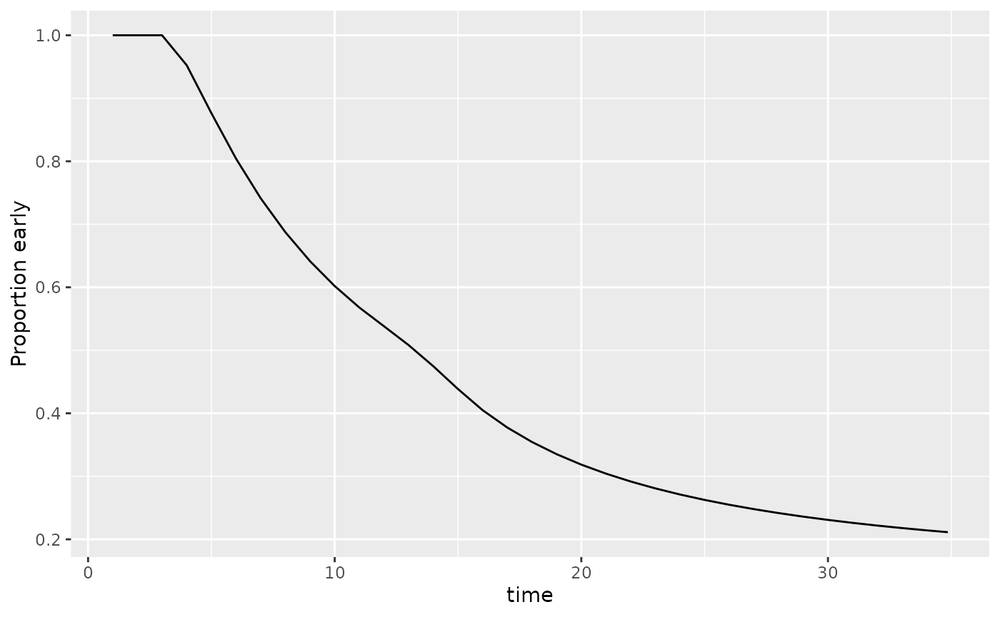

As shown by the above plot, the IA1 analysis time is 19.1. With the IA1 analysis time known, we now derive the group sequential design with the futility bound by Korn and Freidlin (2018).

kf <- gs_power_ahr(
  enroll_rate = enroll_rate, 
  fail_rate = fail_rate,
  ratio = ratio,
  # 2 IAs + 1 FA
  event = 512 * c(.5, .75, 1),
  analysis_time = c(ia1_time, 
                    ia1_time + 0.01, 
                    ia1_time + 0.02),
  # efficacy bound
  upper = gs_b, 
  upar = c(Inf, Inf, qnorm(.975)),
  # futility bound
  lower = gs_b, 
  lpar = c(0, 0, -Inf))

kf |>
  summary() |>
  as_gt(title = "Group sequential design with futility only",
        subtitle = "Korn and Freidlin futility rule stops if HR > 1")

Bound	Z	Nominal p¹	~HR at bound²	Cumulative boundary crossing probability
Group sequential design with futility only
Korn and Freidlin futility rule stops if HR > 1
Bound	Z	Nominal p¹	~HR at bound²	Alternate hypothesis	Null hypothesis
Analysis: 1 Time: 19.1 N: 680 Events: 324.6 AHR: 0.78 Information fraction: 0.63
Futility	0.00	0.500	1.0000	0.0143	0.5000
Analysis: 2 Time: 22.9 N: 680 Events: 384 AHR: 0.77 Information fraction: 0.75
Futility	0.00	0.500	1.0000	0.0152	0.5644
Analysis: 3 Time: 34.9 N: 680 Events: 512 AHR: 0.75 Information fraction: 1
Efficacy	1.96	0.025	0.8409	0.9015	0.0250
¹ One-sided p-value for experimental vs control treatment. Value < 0.5 favors experimental, > 0.5 favors control.
² Approximate hazard ratio to cross bound.

Classical beta-spending futility bound

A classical \(\beta-\)spending bound would assume a constant treatment effect over time using the proportional hazards assumption. We use the average hazard ratio at the fixed design analysis for this purpose.

betaspending_classic <- gs_power_ahr(
  enroll_rate = enroll_rate,
  fail_rate = define_fail_rate(duration = Inf, 
                               fail_rate = -log(.5) / 12,
                               hr = fixedevents$analysis$ahr,
                               dropout_rate = 0),
  ratio = ratio,
  # 2 IAs + 1 FA
  event = 512 * c(.5, .75, 1),
  # efficacy bound
  upper = gs_b,
  upar = c(rep(Inf, 2), qnorm(.975)),
  # futility bound
  lower = gs_spending_bound,
  lpar = list(sf = gsDesign::sfLDOF, total_spend = 0.025, param = NULL, timing = NULL),
  test_lower = c(TRUE, TRUE, FALSE)
)

betaspending_classic |>
  summary() |>
  as_gt(
    title = "Group sequential design with futility only",
    subtitle = "Classical beta-spending futility bound"
  )

Bound	Z	Nominal p¹	~HR at bound²	Cumulative boundary crossing probability
Group sequential design with futility only
Classical beta-spending futility bound
Bound	Z	Nominal p¹	~HR at bound²	Alternate hypothesis	Null hypothesis
Analysis: 1 Time: 15.7 N: 680 Events: 256 AHR: 0.75 Information fraction: 0.5
Futility	-0.68	0.7503	1.0881	0.0015	0.2497
Analysis: 2 Time: 22.9 N: 680 Events: 384 AHR: 0.75 Information fraction: 0.75
Futility	0.46	0.3235	0.9543	0.0095	0.6795
Analysis: 3 Time: 34.4 N: 680 Events: 512 AHR: 0.75 Information fraction: 1
Efficacy	1.96	0.0250	0.8409	0.9037	³ 0.0249
¹ One-sided p-value for experimental vs control treatment. Value < 0.5 favors experimental, > 0.5 favors control.
² Approximate hazard ratio to cross bound.
³ Cumulative alpha for final analysis (0.0249) is less than the full alpha (0.025) when the futility bound is non-binding. The smaller value subtracts the probability of crossing a futility bound before crossing an efficacy bound at a later analysis (0.025 - 0.0001 = 0.0249) under the null hypothesis.

Conclusion

As an alternative ad hoc methods to account for delayed effects as proposed by Wieand, Schroeder, and O’Fallon (1994) and Korn and Freidlin (2018), we propose a method for \(\beta\)-spending that automatically accounts for delayed effects. We have shown that results compare favorably to the ad hoc methods, but control Type II error and adapt to the timing and distribution of event times at the time of interim analysis.

References

Chen, Tai-Tsang. 2013. “Statistical Issues and Challenges in Immuno-Oncology.” Journal for ImmunoTherapy of Cancer 1 (18): 1–9.

Korn, Edward L, and Boris Freidlin. 2018. “Interim Futility Monitoring Assessing Immune Therapies with a Potentially Delayed Treatment Effect.” Journal of Clinical Oncology 36 (23): 2444–49.

Wieand, Sam, Georgene Schroeder, and Judith Rich O’Fallon. 1994. “Stopping When the Experimental Regimen Does Not Appear to Help.” Statistics in Medicine 13 (13-14): 1453–58.