Simulating time-to-event trials in parallel

Overview

This vignette demonstrates the ability to implement sim_fixed_n() using user-defined backends to parallelize simulations. We will consider the backends supported by the future framework.

The backends supported by the future package include:

sequential - default and non-parallel backend.
multisession - uses multiple background R sessions on a single machine.
multicore - uses multiple forked R processes on a single non-Windows machine outside of RStudio.
cluster - supports external R sessions across multiple machines.

You can also choose other backend types supported by additional future extension packages, such as the HPC job scheduler backends from future.batchtools.

The function sim_fixed_n() provides a simulation workflow for a two-arm trial with a single endpoint. We can vary the parameters of the trial using different functions outlined in the documentation. This function now provides users the opportunity to implement their simulations using the previously described parallel backends to accelerate the computation.

The function sim_gs_n() which simulates group sequential designs under a fixed sample size also supports the use of user-defined backends to parallelize simulations in a similar manner.

Background

Without specifying a backend, sim_fixed_n() will execute sequentially. The sequential execution will run all n_sim iterations within the same process or session of R. In order to execute in parallel, we must define the environment prior to calling the function. Setting your seed prior to calling the function will ensure that the results are reproducible.

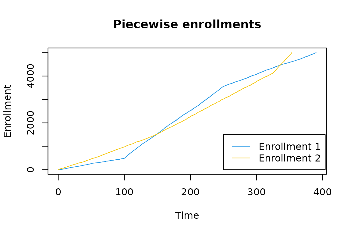
Suppose you want to investigate the duration of a trial under two possible enrollments strategies. Both enrollments are piecewise, but have varying durations and rates.

library(simtrial)
library(future)
library(doFuture)

set.seed(1)

n <- 5000
enroll_rate1 <- data.frame(rate = c(5, 20, 10), duration = c(100, 150, 150))
enroll_rate2 <- data.frame(rate = c(10, 15, 30), duration = c(150, 175, 75))
x1 <- rpwexp_enroll(n = n, enroll_rate = enroll_rate1)
x2 <- rpwexp_enroll(n = n, enroll_rate = enroll_rate2)

plot(
  x1, 1:n,
  type = "l",
  col = palette()[4],
  xlim = c(0, max(x1, x2)),
  main = "Piecewise enrollments",
  xlab = "Time",
  ylab = "Enrollment"
)
lines(x2, 1:n, col = palette()[7])
legend(
  250, 1500,
  legend = c("Enrollment 1", "Enrollment 2"),
  col = c(palette()[4], palette()[7]),
  lty = c(1, 1)
)

We see that Enrollment 2 enrolls individuals more quickly than Enrollment 1 at onset. Later, Enrollment 1 will outpace Enrollment 2 before eventually being overtaken again. As such, we want to consider how the duration of the study changes under these enrollments.

The sequential run

Naively, we can execute these simulations sequentially. We set the target of a total enrollment of 3000 individuals with the trial ending after observing 700 events. We use timing_type = 2 to return the correct trial duration.

set.seed(1)

n_sim <- 200

start_sequential <- proc.time()

seq_result1 <- sim_fixed_n(
  n_sim = n_sim,
  sample_size = 3000,
  target_event = 700,
  enroll_rate = enroll_rate1,
  timing_type = 2 # Time until targeted event count achieved
)
#> Backend uses sequential processing.

seq_result2 <- sim_fixed_n(
  n_sim = n_sim,
  sample_size = 3000,
  target_event = 700,
  enroll_rate = enroll_rate2,
  timing_type = 2 # Time until targeted event count achieved
)
#> Backend uses sequential processing.

duration_sequential <- proc.time() - start_sequential

A message automatically appears in the console that indicates what backend is being used for processing.

The calls to proc.time() allow us to evaluate the computation time of these procedures. This function provides three outputs, we will focus on user and elapsed time. User time represents the CPU time spent evaluating the function and elapsed time represents the “wall clock” time spent by the end user waiting for the results.

print(duration_sequential)
#>    user  system elapsed 
#>  13.959   0.041   8.070

We can see that the CPU time is 13.96 and the elapsed time is 8.07 seconds. These provide our baseline for the computation time.

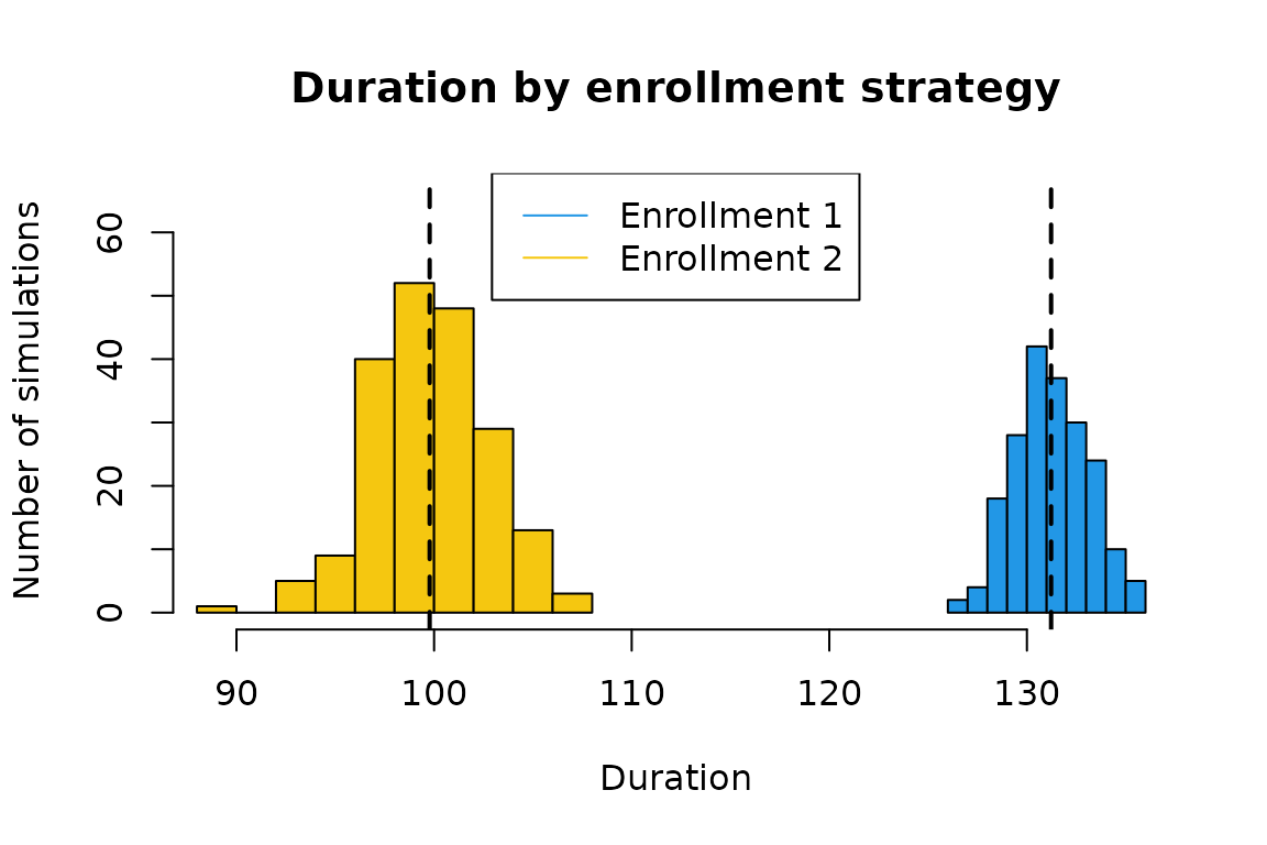
As you may have anticipated, we see that for a lower number of events, enrollment 2 has a shorter average duration of 99.8 over that of enrollment 1, which is 131.2.

We also see that there is a distinction between the duration of the study under the proposed enrollment strategies.

Setting up a parallel backend

If we instead, wanted to run more simulations for each enrollment, we can expect the time to run our simulations to increase. As we vary and increase the number of parameter inputs that we consider, we expect the simulation process to continue to increase in duration. To help combat the growing computational burden, we can run these simulations in parallel using the multisession backend available to us in plan().

We can adjust the default number of cores with the function parallelly::availableCores(). The multisession backend will automatically use all available cores by default, but here we will use two. To initialize our backend, we change our plan.

plan(multisession, workers = 2)

Execution in parallel

Once we have configured the backend details, we can execute the same code as before to automatically distribute the n_sim simulations across the available cores.

set.seed(1)

start_sequential <- proc.time()

seq_result1m <- sim_fixed_n(
  n_sim = n_sim,
  sample_size = 3000,
  target_event = 700,
  enroll_rate = enroll_rate1,
  timing_type = 2 # Time until targeted event count achieved
)
#> Using 2 cores with backend multisession

seq_result2m <- sim_fixed_n(
  n_sim = n_sim,
  sample_size = 3000,
  target_event = 700,
  enroll_rate = enroll_rate2,
  timing_type = 2 # Time until targeted event count achieved
)
#> Using 2 cores with backend multisession

duration_sequential <- proc.time() - start_sequential

print(duration_sequential)
#>    user  system elapsed 
#>   0.425   0.012   7.681

We can see that the CPU time is 0.42 and the elapsed time is 7.68 seconds. The user time here appears to be drastically reduced because of how R keeps track of time; the time used by the parent process and not the children processes are reported for the user time. Therefore, we compare the elapsed time to see the real-world impact of the parallelization.

To change the implementation back to a sequential backend, we simply use what is below.

plan(sequential)

We can also verify that the simulation results are identical because of setting a seed and that the backend type will not affect the results. Below, it is clear that the results from our sequential and multisession backends match completely.

sum(seq_result1 != seq_result1m)
sum(seq_result2 != seq_result2m)

Note: A parallel implementation may not always be faster than a serial implementation. If there is substantial overhead associated with executing in parallel, sequential evaluation may be faster. For a low number of simulations or available cores, it may be preferable to continue computation in serial rather than parallel. We leave it to the end user to determine this difference based on the resources available to them.

A nested parallel example

We provide an additional example using a nested parallel structure for users with more extensive resources, such as high-performance computing clusters, available to them. Because these resources are not commonly available, we will not execute the below code herein. Consider that you have two accessible nodes, each with three cores (shown in the diagram below).

Available resource schematic.

Ideally, all available resources will be used when executing the simulations. To do this, we need to correctly define our backend using plan() and run the same code as previously. The different structures, or topologies, for a backend can be changed with a more in depth explanation given in the future topologies vignette. Our below example follows closely their example.

In our below snippet, we consider the two nodes named n1 and n2 and create a function to select the number of cores to use on those named nodes. While trivial here, a courteous user of shared machines would specify fewer than all available cores and can do such using a modification of the below code. We then implement our backend using a list that follows the hierarchy of the available resources.

nodes <- c("n1", "n2")
custom_cores <- function() {
  switch(Sys.info()[["nodename"]],
    "n1" = 3L, # Modify here for number of cores on node1
    "n2" = 3L, # Modify here for number of cores on node2
    ## Default:
    availableCores()
  )
}
plan(list(
  tweak(cluster, workers = nodes),
  tweak(multisession, workers = custom_cores)
))

The function tweak() is necessary to override the inherent protection of nested parallelism, meant to help avoid overloading one’s resources by errantly starting too many processes. Because of the need to tweak backends, the message echoed to the console for nested backends reflects the highest level of the nested hierarchy.

With the backend in place, we then can run the identical code from before using all available resources and return the same results as before.

set.seed(1)

enroll_rates <- list(enroll_rate1, enroll_rate2)

seq_resultc <- foreach::foreach(
  i = 1:2,
  .combine = "list",
  .options.future = list(seed = TRUE)
) %dofuture% {
  sim_fixed_n(
    n_sim = n_sim,
    sample_size = 3000,
    target_event = 700,
    enroll_rate = enroll_rates[[i]],
    timing_type = 2 # Time until targeted event count achieved
  )
}

Then, we reset the plan to sequential to avoid accidentally continuing to execute later calls within these resources.