Simulate Fixed Designs with Ease via sim_fixed_n

Yujie Zhao and Keaven Anderson

library(gsDesign2)
library(simtrial)
library(dplyr)
library(gt)

set.seed(2027)

The sim_fixed_n() function simulates a two-arm trial with a single endpoint, accounting for time-varying enrollment, hazard ratios, and failure and dropout rates.

While there are limitations, there are advantages of calling sim_fixed_n() directly:

• It is simple, which allows for a single function call to perform an arbitrary number of simulations.
• It automatically implements a parallel computating backend to reduce running time.
• It offers up to 5 options for determining the data cutoff for analysis through the timing_type parameter.

If people are interested in more complicated simulations, please refer to the vignette Custom Fixed Design Simulations: A Tutorial on Writing Code from the Ground Up.

The process for simulating via sim_fixed_n() is outlined in Steps 1 to 3 below.

Step 1: Define design parameters

To run simulations for a fixed design, several design characteristics may be used. Depending on the data cutoff for analysis option, different inputs may be required. The following lines of code specify an unstratified 2-arm trial with equal randomization. The simulation is repeated 2 times. Enrollment is targeted to last for 12 months at a constant enrollment rate. The median for the control arm is 10 months, with a delayed effect during the first 3 months followed by a hazard ratio of 0.7 thereafter. There is an exponential dropout rate of 0.001 over time.

n_sim <- 100
total_duration <- 36
stratum <- data.frame(stratum = "All", p = 1)
block <- rep(c("experimental", "control"), 2)

enroll_rate <- data.frame(stratum = "All", rate = 12, duration = 500 / 12)
fail_rate <- data.frame(stratum = "All",
                        duration = c(3, Inf), fail_rate = log(2) / 10, 
                        hr = c(1, 0.6), dropout_rate = 0.001)

We specify sample size and targeted event count based on the fixed_design_ahr() function and the above options. The following design computes the sample size and targeted event counts for 85% power. In this approach, users can obtain the sample size and targeted events from the output of x, specifically by using sample_size <- x$analysis$n and target_event <- x$analysis$event.

x <- fixed_design_ahr(enroll_rate = enroll_rate, fail_rate = fail_rate, 
                      alpha = 0.025, power = 0.85, ratio = 1, 
                      study_duration = total_duration) |> to_integer()
x |> summary() |> gt() |> 
  tab_header(title = "Sample Size and Targeted Events Based on AHR Method", 
             subtitle = "Fixed Design with 85% Power, One-sided 2.5% Type I error") |>
  fmt_number(columns = c(4, 5, 7), decimals = 2)

Sample Size and Targeted Events Based on AHR Method
Fixed Design with 85% Power, One-sided 2.5% Type I error
Design	N	Events	Time	Bound	alpha	Power
Average hazard ratio	516	295	36.01	1.96	0.025	0.85

Now we set the derived targeted sample size, enrollment rate, and event count from the above.

sample_size <- x$analysis$n
target_event <- x$analysis$event
enroll_rate <- x$enroll_rate

Step 2: Run sim_fixed_n()

Now that we have set up the design characteristics in Step 1, we can proceed to run sim_fix_n() for our simulations. This function automatically utilizes a parallel computing backend, which helps reduce the running time.

The timing_type specifies one or more of the following cutoffs for setting the time for analysis:

• timing_type = 1: The planned study duration.
• timing_type = 2: The time until target event count has been observed.
• timing_type = 3: The planned minimum follow-up period after enrollment completion.
• timing_type = 4: The maximum of planned study duration and time to observe the targeted event count (i.e., using timing_type = 1 and timing_type = 2 together).
• timing_type = 5: The maximum of time to observe the targeted event count and minimum follow-up following enrollment completion (i.e., using timing_type = 2 and timing_type = 3 together).

The rho_gamma argument is a data frame containing the variables rho and gamma, both of which should be greater than or equal to zero, to specify one Fleming-Harrington weighted log-rank test per row. For instance, setting rho = 0 and gamma = 0 yields the standard unweighted log-rank test, while rho = 0 and gamma = 0.5 provides the weighted Fleming-Harrington (0, 0.5) log-rank test. If you are interested in tests other than the Fleming-Harrington weighted log-rank test, please refer to the vignette Custom Fixed Design Simulations: A Tutorial on Writing Code from the Ground Up.

sim_res <- sim_fixed_n(
  n_sim = 2, # only use 2 simulations for initial run
  sample_size = sample_size, 
  block = block, 
  stratum = stratum,
  target_event = target_event, 
  total_duration = total_duration,
  enroll_rate = enroll_rate, 
  fail_rate = fail_rate,
  timing_type = 1:5, 
  rho_gamma = data.frame(rho = 0, gamma = 0))

The output of sim_fixed_n is a data frame with one row per simulated dataset per cutoff specified in timing_type, per test statistic specified in rho_gamma. Here we have just run 2 simulated trials and see how the different cutoffs vary for the 2 trial instances.

sim_res |>
  gt() |>
  tab_header("Tests for Each Simulation Result", subtitle = "Logrank Test for Different Analysis Cutoffs") |>
  fmt_number(columns = c(4, 5, 7), decimals = 2)

Tests for Each Simulation Result
Logrank Test for Different Analysis Cutoffs
method	parameter	estimate	se	z	event	ln_hr	cut	duration	sim
WLR	FH(rho=0, gamma=0)	-31.52010	8.38	3.76	287	−0.45	Planned duration	36.00000	1
WLR	FH(rho=0, gamma=0)	-32.12426	8.49	3.78	295	−0.45	Targeted events	36.66316	1
WLR	FH(rho=0, gamma=0)	-29.13247	8.25	3.53	278	−0.43	Minimum follow-up	35.20859	1
WLR	FH(rho=0, gamma=0)	-32.12426	8.49	3.78	295	−0.45	Max(planned duration, event cut)	36.66316	1
WLR	FH(rho=0, gamma=0)	-32.12426	8.49	3.78	295	−0.45	Max(min follow-up, event cut)	36.66316	1
WLR	FH(rho=0, gamma=0)	-31.88270	8.00	3.99	268	−0.50	Planned duration	36.00000	2
WLR	FH(rho=0, gamma=0)	-38.09785	8.40	4.54	295	−0.54	Targeted events	38.32488	2
WLR	FH(rho=0, gamma=0)	-34.29092	8.23	4.17	283	−0.51	Minimum follow-up	37.47843	2
WLR	FH(rho=0, gamma=0)	-38.09785	8.40	4.54	295	−0.54	Max(planned duration, event cut)	38.32488	2
WLR	FH(rho=0, gamma=0)	-38.09785	8.40	4.54	295	−0.54	Max(min follow-up, event cut)	38.32488	2

Step 3: Summarize simulations

Now we run 100 simulated trials and summarize the results by how data is cutoff for analysis.

sim_res <- sim_fixed_n(
  n_sim = n_sim,
  sample_size = sample_size, 
  block = block, stratum = stratum,
  target_event = target_event, 
  total_duration = total_duration,
  enroll_rate = enroll_rate, 
  fail_rate = fail_rate,
  timing_type = 1:5, 
  rho_gamma = data.frame(rho = 0, gamma = 0))

With the 100 simulations provided, users can summarize the simulated power and compare it to the targeted 85% power. All cutoff methods approximate the targeted power well and have a similar average duration and mean number of events.

sim_res |>
  group_by(cut) |>
  summarize(`Simulated Power` = mean(z > qnorm(1 - 0.025)), 
            `Mean events` = mean(event),
            `Mean duration` = mean(duration)) |>
  mutate(`Sample size` = sample_size,
         `Targeted events` = target_event) |>
  gt() |>
  tab_header(title = "Summary of 100 simulations by 5 different analysis cutoff methods",
             subtitle = "Tested by logrank") |>
  fmt_number(columns = c(2:4), decimals = 2)

Summary of 100 simulations by 5 different analysis cutoff methods
Tested by logrank
cut	Simulated Power	Mean events	Mean duration	Sample size	Targeted events
Max(min follow-up, event cut)	0.85	299.35	36.39	516	295
Max(planned duration, event cut)	0.85	301.54	36.59	516	295
Minimum follow-up	0.84	291.57	35.78	516	295
Planned duration	0.84	294.74	36.00	516	295
Targeted events	0.85	295.00	36.00	516	295

We can also do things like summarize distribution of event counts at the planned study duration. We can see the event count varies a fair amount.

hist(sim_res$event[sim_res$cut == "Planned duration"], 
     breaks = 10,
     main = "Distribution of Event Counts at Planned Study Duration",
     xlab = "Event Count at Targeted Trial Duration")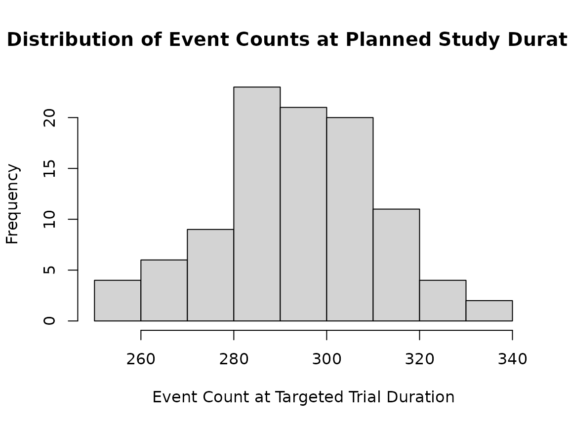

We also evaluate the distribution of the trial duration when analysis is performed when the targeted events are achieved.

plot(density(sim_res$duration[sim_res$cut == "Targeted events"]), 
     main = "Trial Duration Smoothed Density",
     xlab = "Trial duration when Targeted Event Count is Observed")