Design Using Average Hazard Ratio

# packages used
library(gsDesign)
library(gsDesign2)
library(gsdmvn)
library(ggplot2)
library(dplyr)
library(knitr)
library(kableExtra)
library(gt)
library(tidyr)

Introduction

Jennison and Turnbull (2000)

Scenarios

Expected enrollment duration is 24 months with piecewise constant enrollment rates escalating every 2 months until month 6 where enrollment is assumed to have reached steady state. For alternate scenarios, enrollment will occur at a faster than planned rate. For both scenarios, we assume for initial illustrations that the total enrollment is 100 subjects.

# 6 month ramp-up of enrollment, 24 months enrollment time target
enroll24 <- tibble::tibble(Stratum = rep("All",4), 
                           duration = c(rep(2,3), 18),
                           rate = 1:4)
# Set rates to enroll 100 subjects
N <- sum(enroll24$duration * enroll24$rate)
enroll24$rate <- enroll24$rate * 100 / N

# Enroll in 16 months, same ramp-up
enroll16 <- tibble::tibble(Stratum = rep("All",4), 
                           duration = c(rep(2,3), 12),
                           rate = 1:4)
# Set rates to enroll 100 subjects
N <- sum(enroll16$duration * enroll16$rate)
enroll16$rate <- enroll16$rate * 100 / N
# Put these in a single tibble by scenario
# We will use 16 month enrollment for delayed effect and crossing hazards
# scenarios
enrollRates <- rbind(enroll24 %>% mutate(Scenario = "PH"),
                     enroll24 %>% mutate(Scenario = "Delayed effect 1"),
                     enroll16 %>% mutate(Scenario = "Delayed effect 2"),
                     enroll16 %>% mutate(Scenario = "Crossing")
)

We will consider the following failure rate assumptions:

PH: Proportional hazards is assumed.
- Control group has exponential failure rate with a median of 12 months.
- Constant hazard ratio of 0.7 (experimental/control).
Delayed effect
- Control group has exponential failure rate with a median of 10 months.
- Hazard ratio of 1 for 6 months followed by a hazard ratio of 0.575.
Crossing hazards
- Control group has exponential failure rate with a median of 10 months.
- Hazard ratio of 1.5 for 4 months followed by a hazard ratio of 0.5.

Survival curves for these 3 scenarios are shown below:

Month <- c(0,4,6,44)
duration <- Month - c(0,Month[1:3])
control_rate <- log(2) / c(rep(16,4), rep(14, 4), rep(14, 4))
s <- tibble::tibble(Scenario = c(rep("PH",4), rep("Delayed effect", 4), rep("Crossing", 4)),
                    Treatment = rep("Control", 12),
                    Month = rep(Month, 3),
                    duration = rep(duration, 3),
                    rate = control_rate,
                    hr = c(rep(.7, 4), c(1, 1, 1, .575), c(1.5,1.5, .5, .5)),
)
s <- rbind(s,
           s %>% mutate(Treatment = "Experimental",
                        rate = rate * hr)
) %>%
  group_by(Scenario, Treatment) %>%
  mutate(Survival = exp(-cumsum(duration * rate)))
ggplot(s, aes(x = Month, y = Survival, col = Scenario, lty = Treatment)) + 
  geom_line() +
  scale_y_log10(breaks = (1:10) /10, lim=c(.1,1))+
  scale_x_continuous(breaks = seq(0,42, 6))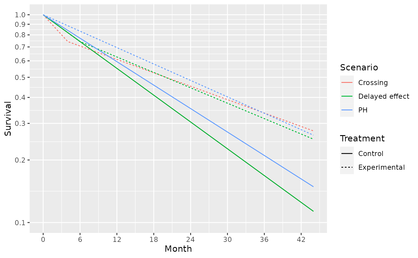

Average Hazard Ratio

# Durations to be used in common for all failure rate scenarios
dur <- c(4,2,100)
# Exponential failure, proportional hazards
failRates <- rbind(tibble(Scenario = "PH", Stratum = "All", 
                          duration = dur, failRate = log(2) / 14,
                          hr = 0.7, dropoutRate = .001),
                   tibble(Scenario = "Delayed effect 1", Stratum = "All", 
                          duration = dur, failRate = log(2) / 11,
                          hr = c(1, .6, .6), dropoutRate = .001),
                   tibble(Scenario = "Delayed effect 2", Stratum = "All", 
                          duration = dur, failRate = log(2) / 11,
                          hr = c(1, 1, .7), dropoutRate = .001),
                   tibble(Scenario = "Crossing", Stratum = "All", 
                          duration = dur, failRate = log(2) / 11,
                          hr = c(1.5, .6,.6), dropoutRate = .001)
)
hr <- NULL
for(g in c("PH", "Delayed effect 1", "Delayed effect 2", "Crossing")){
  hr <- 
    rbind(hr,
        AHR(enrollRates = enrollRates %>% filter(Scenario == g), 
            failRates = failRates %>% filter(Scenario == g),
            totalDuration = c(.001, seq(4, 44, 4))
        ) %>%
        mutate(Scenario = g)
  )
}

ggplot(hr, aes(x=Time, y=AHR, col = Scenario)) + geom_line() + scale_x_continuous(breaks = seq(0, 42, 6))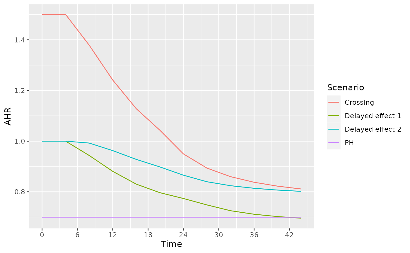

ggplot(hr, aes(x=Time, y=`Events`, col = Scenario)) + geom_line() + scale_x_continuous(breaks = seq(0, 42, 6))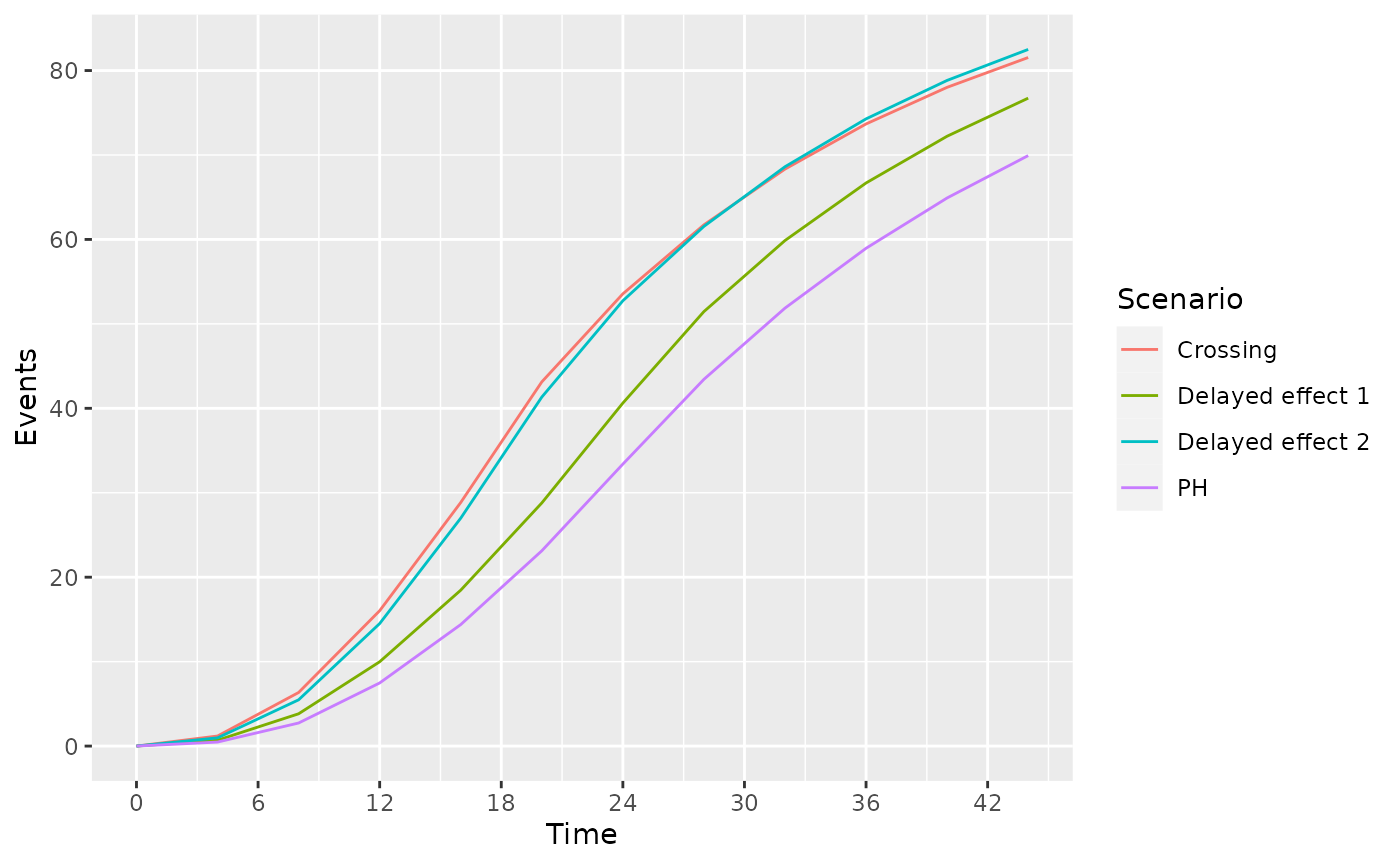

Sample Size and Events by Scenario

Fixed design using AHR and logrank

We power a fixed design at 90% with 2.5% one-sided Type I error under the different scenarios under consideration.

ss_ahr_fixed <- NULL
for(g in c("PH", "Delayed effect 1","Delayed effect 2", "Crossing")){
    ss_ahr_fixed <- 
      rbind(ss_ahr_fixed,
      gs_design_ahr(enrollRates = enrollRates %>% filter(Scenario == g),
                    failRates = failRates %>% filter(Scenario == g),
                    analysisTimes = 36,
                    upper = gs_b, upar = qnorm(.975),
                    lower = gs_b, lpar = -Inf,
                    alpha = .025,
                    beta = .1
                    )$bounds %>% mutate(Scenario = g)
      )
}
ss_ahr_fixed %>% select(Time, N, Events, AHR, Scenario) %>% 
  gt() %>% fmt_number(columns=1:3,decimals = 0) %>% fmt_number(columns = 4, decimals = 3)  %>%
  tab_header(title = "Sample Size and Events Required by Scenario",
             subtitle = "36 Month Trial duration, 2.5% One-sided Type 1 Error, 90% Power")

Time	N	Events	AHR	Scenario
Sample Size and Events Required by Scenario
36 Month Trial duration, 2.5% One-sided Type 1 Error, 90% Power
36	563	332	0.700	PH
36	547	365	0.711	Delayed effect 1
36	1,338	993	0.814	Delayed effect 2
36	1,846	1,360	0.838	Crossing

Assuming delayed effect 1 is the primary scenario for which we wish to protect power, how long should the trial be to optimize the tradeoffs between sample size, AHR and events required? We will inform this tradeoff by looking sizing the trial for different assumed trial durations with the same failure rates and assumed relative enrollment rates. The counts of events required is perhaps the most interesting here in that a 24 month trial requires almost twice the events to be powered at 90% compared to a trial of 42 months duration. For further study, we will consider the 36 month trial duration as a reasonable tradeoff between time, sample size and power under a presumed delayed effect of 4 months followed by a hazard ratio of 0.6 thereafter.

ss_ahr_fixed <- NULL
g <- "Delayed effect 1"
for(trialEnd in c(24,30,36,42)){
    ss_ahr_fixed <- 
      rbind(ss_ahr_fixed,
      gs_design_ahr(enrollRates = enrollRates %>% filter(Scenario == g),
                    failRates = failRates %>% filter(Scenario == g),
                    analysisTimes = trialEnd,
                    upper = gs_b, upar = qnorm(.975),
                    lower = gs_b, lpar = -Inf,
                    alpha = .025,
                    beta = .1
                    )$bounds %>% mutate(Scenario = g)
      )
}
ss_ahr_fixed %>% select(Time, N, Events, AHR, Scenario) %>% 
  gt() %>% fmt_number(columns=1:3,decimals = 0) %>% fmt_number(columns = 4, decimals = 3) %>%
  tab_header(title = "Sample Size and Events Required by Trial Duration",
             subtitle = "Delayed Effect of 4 Months, HR = 0.6 Thereafter; 90% Power")

Time	N	Events	AHR	Scenario
Sample Size and Events Required by Trial Duration
Delayed Effect of 4 Months, HR = 0.6 Thereafter; 90% Power
24	1,582	643	0.774	Delayed effect 1
30	801	448	0.735	Delayed effect 1
36	547	365	0.711	Delayed effect 1
42	441	329	0.699	Delayed effect 1

Alternate hypothesis mapping

Experimental version of AHR().

AHRx <- function(enrollRates=tibble::tibble(Stratum="All",
                                           duration=c(2,2,10),
                                           rate=c(3,6,9)),
                failRates=tibble::tibble(Stratum="All",
                                         duration=c(3,100),
                                         failRate=log(2)/c(9,18),
                                         hr=c(.9,.6),
                                         dropoutRate=rep(.001,2)),
                totalDuration=30,
                ratio=1,
                simple=TRUE
){
  # check input values
  # check input enrollment rate assumptions
  if(max(names(enrollRates)=="Stratum") != 1){stop("gsDesign2: enrollRates column names in `AHR()` must contain stratum")}
  if(max(names(enrollRates)=="duration") != 1){stop("gsDesign2: enrollRates column names in `AHR()` must contain duration")}
  if(max(names(enrollRates)=="rate") != 1){stop("gsDesign2: enrollRates column names in `AHR()' must contain rate")}

  # check input failure rate assumptions
  if(max(names(failRates)=="Stratum") != 1){stop("gsDesign2: failRates column names in `AHR()` must contain stratum")}
  if(max(names(failRates)=="duration") != 1){stop("gsDesign2: failRates column names in `AHR()` must contain duration")}
  if(max(names(failRates)=="failRate") != 1){stop("gsDesign2: failRates column names in `AHR()` must contain failRate")}
  if(max(names(failRates)=="hr") != 1){stop("gsDesign2: failRates column names in `AHR()` must contain hr")}
  if(max(names(failRates)=="dropoutRate") != 1){stop("gsDesign2: failRates column names in `AHR()` must contain dropoutRate")}

  # check input trial durations
  if(!is.numeric(totalDuration)){stop("gsDesign2: totalDuration in `AHR()` must be a non-empty vector of positive numbers")}
  if(!is.vector(totalDuration) > 0){stop("gsDesign2: totalDuration in `AHR()` must be a non-empty vector of positive numbers")}
  if(!min(totalDuration) > 0){stop("gsDesign2: totalDuration in `AHR()` must be greater than zero")}
  strata <- names(table(enrollRates$Stratum))
  strata2 <- names(table(failRates$Stratum))
  length(strata) == length(strata2)
  for(s in strata){
    if(max(strata2==s) != 1){stop("gsDesign2: Strata in `AHR()` must be the same in enrollRates and failRates")}
  }
  # check input simple is logical
  if(!is.logical(simple)){stop("gsDesign2: simple in `AHR()` must be logical")}

  # compute proportion in each group
  Qe <- ratio / (1 + ratio)
  Qc <- 1 - Qe

  # compute expected events by treatment group, stratum and time period
  rval <- NULL
  for(td in totalDuration){
    events <- NULL
    for(s in strata){
      # subset to stratum
      enroll <- enrollRates %>% filter(Stratum==s)
      fail <- failRates %>% filter(Stratum==s)
      # Control events
      enrollc <- enroll %>% mutate(rate=rate*Qc)
      control <- eEvents_df(enrollRates=enrollc,failRates=fail,totalDuration=td,simple=FALSE)
      # Experimental events
      enrolle <- enroll %>% mutate(rate=rate*Qe)
      fre <- fail %>% mutate(failRate=failRate*hr)
      experimental <- eEvents_df(enrollRates=enrolle,failRates=fre,totalDuration=td,simple=FALSE)
      # Combine control and experimental; by period recompute HR, events, information
      events <-
        rbind(control %>% mutate(Treatment="Control"),
              experimental %>% mutate(Treatment="Experimental")) %>%
        arrange(t, Treatment) %>% ungroup() %>% group_by(t) %>%
        summarize(Stratum = s, info = (sum(1 / Events))^(-1),
                  Events = sum(Events), HR = last(failRate) / first(failRate)
        ) %>%
        rbind(events)
    }
    rval <- rbind(rval,
                  events %>%
                    mutate(Time=td, lnhr = log(HR), info0 = Events * Qc * Qe) %>%
# NEXT 2 lines are the only changes from AHR()
                    ungroup() %>% group_by(Stratum, t) %>%
                    summarize(Time = td, Events = sum(Events), HR=first(HR), lnhr=first(lnhr), info0 = sum(info0), info = sum(info)) %>% ungroup()
    )
  }

  if(!simple) return(rval %>% select(c("Time", "Stratum", "t", "HR", "Events", "info", "info0")) %>% 
                       group_by(Time, Stratum) %>% arrange(t, .by_group = TRUE))
  return(rval %>%
           group_by(Time) %>%
           summarize(AHR = exp(sum(log(HR)*Events)/sum(Events)),
                     Events = sum(Events),
                     info = sum(info),
                     info0 = sum(info0))
  )
}

Under the different scenarios of interest, we can examine the expected number of events in time periods of interest.

events_by_time_period <- NULL
for(g in c("PH", "Delayed effect 1","Delayed effect 2", "Crossing")){
    events_by_time_period <- 
      rbind(events_by_time_period,
      AHRx(enrollRates = enrollRates %>% filter(Scenario == g),
          failRates = failRates %>% filter(Scenario == g),
          totalDuration = c(12, 20, 28, 36), simple = FALSE) %>% mutate(Scenario = g)
      )
}

## `summarise()` has grouped output by 'Stratum'. You can override using the
## `.groups` argument.
## `summarise()` has grouped output by 'Stratum'. You can override using the
## `.groups` argument.
## `summarise()` has grouped output by 'Stratum'. You can override using the
## `.groups` argument.
## `summarise()` has grouped output by 'Stratum'. You can override using the
## `.groups` argument.
## `summarise()` has grouped output by 'Stratum'. You can override using the
## `.groups` argument.
## `summarise()` has grouped output by 'Stratum'. You can override using the
## `.groups` argument.
## `summarise()` has grouped output by 'Stratum'. You can override using the
## `.groups` argument.
## `summarise()` has grouped output by 'Stratum'. You can override using the
## `.groups` argument.
## `summarise()` has grouped output by 'Stratum'. You can override using the
## `.groups` argument.
## `summarise()` has grouped output by 'Stratum'. You can override using the
## `.groups` argument.
## `summarise()` has grouped output by 'Stratum'. You can override using the
## `.groups` argument.
## `summarise()` has grouped output by 'Stratum'. You can override using the
## `.groups` argument.
## `summarise()` has grouped output by 'Stratum'. You can override using the
## `.groups` argument.
## `summarise()` has grouped output by 'Stratum'. You can override using the
## `.groups` argument.
## `summarise()` has grouped output by 'Stratum'. You can override using the
## `.groups` argument.
## `summarise()` has grouped output by 'Stratum'. You can override using the
## `.groups` argument.

events_by_time_period %>% gt()

t	HR	Events	info	info0	Scenario
12 - All
0	0.7	5.1852619	1.2615254	1.2963155	PH
4	0.7	1.2900768	0.3161088	0.3225192	PH
6	0.7	0.9992867	0.2461646	0.2498217	PH
0	1.0	7.5026311	1.8756578	1.8756578	Delayed effect 1
4	0.6	1.4148718	0.3334561	0.3537179	Delayed effect 1
6	0.6	1.0660140	0.2551204	0.2665035	Delayed effect 1
0	1.0	10.5036835	2.6259209	2.6259209	Delayed effect 2
4	1.0	2.4549051	0.6137263	0.6137263	Delayed effect 2
6	0.7	1.5503657	0.3774733	0.3875914	Delayed effect 2
0	1.5	12.7170764	3.0829595	3.1792691	Crossing
4	0.6	1.8916151	0.4309693	0.4729038	Crossing
6	0.6	1.4223228	0.3303949	0.3555807	Crossing
20 - All
0	0.7	11.0617281	2.6918692	2.7654320	PH
4	0.7	3.8607787	0.9461198	0.9651947	PH
6	0.7	8.2028185	2.0274071	2.0507046	PH
0	1.0	15.9738890	3.9934723	3.9934723	Delayed effect 1
4	0.6	4.2318445	0.9976903	1.0579611	Delayed effect 1
6	0.6	8.5867796	2.0744467	2.1466949	Delayed effect 1
0	1.0	21.5580025	5.3895006	5.3895006	Delayed effect 2
4	1.0	7.3386703	1.8346676	1.8346676	Delayed effect 2
6	0.7	12.4353719	3.0443187	3.1088430	Delayed effect 2
0	1.5	26.0319889	6.3157669	6.5079972	Crossing
4	0.6	5.6575413	1.2894992	1.4143853	Crossing
6	0.6	11.4403357	2.6904019	2.8600839	Crossing
28 - All
0	0.7	15.4257237	3.7546492	3.8564309	PH
4	0.7	6.4314807	1.5761307	1.6078702	PH
6	0.7	21.5768513	5.3488075	5.3942128	PH
0	1.0	22.2370521	5.5592630	5.5592630	Delayed effect 1
4	0.6	7.0488173	1.6619243	1.7622043	Delayed effect 1
6	0.6	22.1716513	5.4012239	5.5429128	Delayed effect 1
0	1.0	22.2370521	5.5592630	5.5592630	Delayed effect 2
4	1.0	9.1570597	2.2892649	2.2892649	Delayed effect 2
6	0.7	30.1523434	7.4217817	7.5380859	Delayed effect 2
0	1.5	26.8302861	6.5109859	6.7075715	Crossing
4	0.6	7.0611116	1.6097430	1.7652779	Crossing
6	0.6	27.8387318	6.6300112	6.9596830	Crossing
36 - All
0	0.7	15.4257237	3.7546492	3.8564309	PH
4	0.7	6.7480926	1.6537787	1.6870231	PH
6	0.7	36.7770862	9.1420106	9.1942716	PH
0	1.0	22.2370521	5.5592630	5.5592630	Delayed effect 1
4	0.6	7.3945534	1.7436142	1.8486384	Delayed effect 1
6	0.6	37.0547447	9.0971239	9.2636862	Delayed effect 1
0	1.0	22.2370521	5.5592630	5.5592630	Delayed effect 2
4	1.0	9.1570597	2.2892649	2.2892649	Delayed effect 2
6	0.7	42.8818670	10.6126866	10.7204667	Delayed effect 2
0	1.5	26.8302861	6.5109859	6.7075715	Crossing
4	0.6	7.0611116	1.6097430	1.7652779	Crossing
6	0.6	39.7839241	9.6020931	9.9459810	Crossing

Recall that our alternate hypothesis assumes no treatment effect (HR=1) for 4 months and then HR = 0.6 thereafter. For any of the above scenarios, if we wish to base a futility bound on this assumption plus the above number of events in the first 4 months and after 4 months, then we can compute the average hazard ratio under the alternate hazard ratio for each scenario at 20 months as follows. You can see that an interim futility spending bound based on the alternate hypothesis can depend fairly heavily on enrollment and the control failure rate. Note also that at the time of interim analysis, the alternate hypothesis AHR can be computed in this same fashion based on observed events by time period. Note that this can be quite different than the scenario HR; e.g., for PH, we assume HR=0.7 throughout, but for the futility bound comparison, we compute blinded AHR that decreases with each analysis under the alternate hypothesis.

# Time periods for each scenario were 0-4, 4-6, and 6+
# Thus H1 has HR as follows
hr1 <- tibble(t = c(0, 4, 6), hr1 = c(1, .6, .6))
ahr_by_analysis <-
  events_by_time_period %>% 
  full_join(hr1) %>%
  group_by(Scenario, Time) %>%
  summarize(AHR1 = exp(sum(Events * log(hr1))/ sum(Events)))

## Joining, by = "t"
## `summarise()` has grouped output by 'Scenario'. You can override using the
## `.groups` argument.

ahr_by_analysis %>% 
  pivot_wider(names_from = Scenario, values_from = AHR1) %>% 
  gt() %>% fmt_number(columns=2:5, decimals = 3)

Time	Crossing	Delayed effect 1	Delayed effect 2	PH
12	0.900	0.881	0.868	0.855
20	0.817	0.797	0.783	0.766
28	0.749	0.748	0.722	0.719
36	0.723	0.711	0.699	0.686

Group sequential design

Here we assume the design is under a delayed effect model where the delay is not too long and the long-term average hazard ratio benefit is strong. proportional hazards scenario, but we look at power under the alternate scenarios. We will plan a 36 month group sequential design under the delayed effect 1 scenario. Interim analyses are planned after 12, 20, and 28 months.

analysisTimes <- c(12, 20, 28, 36)
upar <- list(sf = gsDesign::sfLDOF, total_spend = 0.025, param = NULL, timing = NULL, theta=0)
lpar <- list(sf = gsDesign::sfHSD, total_spend = .1, param = -2, timing = NULL, theta=NULL)
NPHasymmetric <- gs_design_ahr(enrollRates = enrollRates,
                               failRates = failRates,
                               ratio = 1, alpha = .025, beta = 0.1,
                               # Information fraction not required (but available!)
                               analysisTimes = analysisTimes,
                               # Function to enable spending bound
                               upper = gs_spending_bound, lower = gs_spending_bound,
                               # Spending function and parameters used
                               upar = upar, lpar = lpar
)
NPHasymmetric$bounds

## # A tibble: 8 × 11
##   Analysis Bound  Time     N Events      Z  Probability   AHR theta  info info0
##      <int> <chr> <dbl> <dbl>  <dbl>  <dbl>        <dbl> <dbl> <dbl> <dbl> <dbl>
## 1        1 Upper    12  231.   40.3  6.58  0.0000000236   0.7 0.357  9.82  10.1
## 2        2 Upper    20  436.  125.   3.62  0.0492         0.7 0.357 30.5   31.1
## 3        3 Upper    28  577.  236.   2.52  0.577          0.7 0.357 58.1   59.1
## 4        4 Upper    36  769.  358.   1.99  0.900          0.7 0.357 88.2   89.4
## 5        1 Lower    12  231.   40.3 -1.54  0.00391        0.7 0.357  9.82  10.1
## 6        2 Lower    20  436.  125.  -0.265 0.0156         0.7 0.357 30.5   31.1
## 7        3 Lower    28  577.  236.   0.899 0.0429         0.7 0.357 58.1   59.1
## 8        4 Lower    36  769.  358.   1.99  0.1            0.7 0.357 88.2   89.4

By scenario, we now wish to compute the adjusted expected futility bounds and the power implied.

xx <- NULL
lparx <- lpar
for(g in c("PH", "Delayed effect 1","Delayed effect 2", "Crossing")){
  AHR1 <- (filter(ahr_by_analysis, Scenario == g))$AHR1
  lparx$theta1 <- -log(AHR1)
  yy <- gs_power_ahr(enrollRates = enrollRates %>% filter(Scenario == g),
               failRates = failRates %>% filter(Scenario == g), 
               events = NULL,
               analysisTimes = c(12,20,28,36),
               upper = gs_spending_bound,
               upar = upar,
               lower = gs_spending_bound,
               lpar = lparx)
  xx <- rbind(xx, yy %>% mutate(Scenario = g))
}

Weighted logrank

ss_FH05_fixed <- NULL
g <- "Delayed effect"
# for(g in c("PH", "Delayed effect", "Crossing")){
#     ss_FH05_fixed <- 
#       rbind(ss_FH05_fixed,
    gs_arm <- gsdmvn:::gs_create_arm(enrollRates, failRates %>% filter(Scenario == g), 
                                     ratio = 1,       # Randomization ratio
                                     total_time = 44) # Total study duration
    arm0 <- gs_arm[["arm0"]]
    arm1 <- gs_arm[["arm1"]]
    npsurvSS::size_two_arm(arm0, arm1, power = 0.9, alpha = 0.025, 
                           test = list(test="weighted logrank", weight = "FH_p.5_q0"))
    
    npsurvSS::size_two_arm(arm0, arm1, power = 0.9, alpha = 0.025, 
                       test = list(test="rmst difference", 
                       # Milestone allow user to define RMST cutpoint
                       milestone = 44)) # 42 selected since better than 40 or 44
    gsdmvn:::gs_design_wlr(enrollRates = enrollRates, 
                           failRates = failRates %>% filter(Scenario == g), 
                           weight = function(x, arm0, arm1){
                                      gsdmvn:::wlr_weight_fh(x, arm0, arm1, 
                                                             rho = 0, gamma = 0.5, tau = 4)},
                           alpha = .025, beta = .1,
                           upar = qnorm(.975),
                           lpar = -Inf,
                           analysisTimes = 44)$bounds %>% filter(Bound =="Upper")

# Ignore tau or (tau can be -1) 
gsdmvn:::gs_design_wlr(enrollRates = enrollRates, 
                       failRates = failRates %>% filter(Scenario == g), 
                       weight = function(x, arm0, arm1){
                                  gsdmvn:::wlr_weight_fh(x, arm0, arm1, 
                                                         rho = 0, gamma = 0.5)},
                       alpha = .025, beta = .1,
                       upar = qnorm(.975),
                       lpar = -Inf,
                       analysisTimes = 44)$bounds %>% filter(Bound =="Upper")

# MaxCombo
   MC_test <- data.frame(rho = c(0, 0, .5), gamma = c(0, .5, .5), tau = -1,
                      test = 1:3,
                      Analysis = 1,
                      analysisTimes = 44)
   gs_design_combo(enrollRates,
               failRates %>% filter(Scenario == g),
               MC_test,
               alpha = 0.025,
               beta = 0.1,
               ratio = 1,
               binding = FALSE,
               upper = gs_spending_combo,
               upar = list(sf = gsDesign::sfLDOF, total_spend = 0.025),
               lower = gs_spending_combo,
               lpar = list(sf = gsDesign::sfLDOF, total_spend = .1)
               )
}

References

Jennison, Christopher, and Bruce W. Turnbull. 2000. Group Sequential Methods with Applications to Clinical Trials. Boca Raton, FL: Chapman; Hall/CRC.

Keaven M. Anderson

12/21/2020