Adjusted Sequential p-values

Introduction

This vignette demonstrates the calculation of adjusted sequential p-values for multiple populations in a group sequential trial design. We’ll show a streamlined approach using helper functions to reduce code repetition while maintaining technical accuracy. The methods implemented in this vignette are based on the work by Zhao et al. (2025). The end result is a adjusted p-value at both interim and final analysis for each hypothesis tested. In all cases, this adjusted p-value can be compared to the family-wise error rate (FWER) for the trial simplifying interpretation by adjusting for multiplicity created by testing multiple hypotheses at group sequential analyses.

library(wpgsd)
library(dplyr)
library(purrr)
library(tibble)
library(gt)
library(gsDesign)
library(gMCPLite)

Example Overview

In a 2-arm controlled clinical trial with one primary endpoint, there are 3 null hypotheses based on populations defined defined by biomarker status. In each case the null hypothesis assumes no difference in the distribution of the time until a primary endpoint is reached between the treatment and control groups:

H1: Biomarker A positive population
H2: Biomarker B positive population
H3: Overall population

Multiplicity Strategy

We will use a graphical approach to visualize the multiplicity strategy.

# Transition matrix and initial weights
m <- matrix(c(
  0, 3 / 7, 4 / 7,
  3 / 7, 0, 4 / 7,
  0.5, 0.5, 0
), nrow = 3, byrow = TRUE)

w <- c(0.3, 0.3, 0.4) # Initial weights

# Visualize strategy
name_hypotheses <- c("H1: Biomarker A positive", "H2: Biomarker B positive", "H3: Overall Population")

hplot <- gMCPLite::hGraph(
  3,
  alphaHypotheses = w, m = m,
  nameHypotheses = name_hypotheses, trhw = .2, trhh = .1,
  digits = 5, trdigits = 3, size = 5, halfWid = 1, halfHgt = 0.5,
  offset = 0.2, trprop = 0.4,
  fill = as.factor(c(2, 3, 1)),
  palette = c("#BDBDBD", "#E0E0E0", "#EEEEEE"),
  wchar = "w"
)
hplot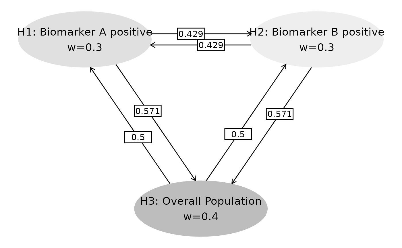

Study Setup

We assume 2 analyses: an interim analysis (IA) and a final analysis (FA). For the multiplicity adjustments, we need the number of events in the treatment and control groups combined that are available for testing each hypothesis at both analyses for each population and the intersection of populations. In the following AB positive means positive for both biomarker A and biomarker B.

# Create event data systematically
create_event_data <- function() {
  populations <- rep(c("A positive", "B positive", "AB positive", "overall"), 2)
  analyses <- rep(c(1, 2), each = 4)
  events <- c(100, 110, 80, 225, 200, 220, 160, 450) # IA, then FA

  tibble(
    population = populations,
    analysis = analyses,
    event = events
  )
}

event_tbl <- create_event_data()
event_tbl %>%
  gt() %>%
  tab_header(title = "Event Count by Population and Analysis")

population	analysis	event
Event Count by Population and Analysis
A positive	1	100
B positive	1	110
AB positive	1	80
overall	1	225
A positive	2	200
B positive	2	220
AB positive	2	160
overall	2	450

We assume the following unadjusted p-values at each analysis for each hypothesis.

# Observed p-values
obs_tbl <- tribble(
  ~hypothesis, ~analysis, ~obs_p,
  "H1", 1, 0.02,
  "H2", 1, 0.01,
  "H3", 1, 0.012,
  "H1", 2, 0.015,
  "H2", 2, 0.012,
  "H3", 2, 0.010
) %>%
  mutate(obs_Z = -qnorm(obs_p))

obs_tbl %>%
  gt() %>%
  tab_header(title = "Nominal p-values")

hypothesis	analysis	obs_p	obs_Z
Nominal p-values
H1	1	0.020	2.053749
H2	1	0.010	2.326348
H3	1	0.012	2.257129
H1	2	0.015	2.170090
H2	2	0.012	2.257129
H3	2	0.010	2.326348


p_obs_IA <- (obs_tbl %>% filter(analysis == 1))$obs_p
p_obs_FA <- (obs_tbl %>% filter(analysis == 2))$obs_p

We now have all the information we need to perform testing and adjusting p-values.

Information Fractions

Next we calculate information fractions at interim and final analyses. The final event count at each analysis is assumed to be the planned count for each population.

# Helper function to extract events
get_events <- function(analysis_num, population_name) {
  event_tbl %>%
    filter(analysis == analysis_num, population == population_name) %>%
    pull(event)
}

# Extract event counts
events_IA <- event_tbl %>% filter(analysis == 1)
events_FA <- event_tbl %>% filter(analysis == 2)

a_pos_IA <- get_events(1, "A positive")
b_pos_IA <- get_events(1, "B positive")
ab_pos_IA <- get_events(1, "AB positive")
overall_IA <- get_events(1, "overall")

a_pos_FA <- get_events(2, "A positive")
b_pos_FA <- get_events(2, "B positive")
ab_pos_FA <- get_events(2, "AB positive")
overall_FA <- get_events(2, "overall")

# Calculate information fractions
IF_IA <- c(
  (a_pos_IA + overall_IA) / (a_pos_FA + overall_FA), # H1
  (b_pos_IA + overall_IA) / (b_pos_FA + overall_FA), # H2
  (ab_pos_IA + overall_IA) / (ab_pos_FA + overall_FA) # H3
)

tibble(
  Hypothesis = c("H1", "H2", "H3"),
  Information_Fraction = IF_IA
) %>%
  gt() %>%
  tab_header(title = "Information Fractions at Interim Analysis") %>%
  fmt_number(columns = 2, decimals = 3)

Hypothesis	Information_Fraction
Information Fractions at Interim Analysis
H1	0.500
H2	0.500
H3	0.500

Correlation Matrix

Now we can create a correlation matrix for all tests performed based on the methods of Anderson et al. (2022) (or Chen et al. (2021)).

# Create correlation matrix using event intersections
event_intersections <- tribble(
  ~H1, ~H2, ~Analysis, ~Event,
  # Analysis 1 - Interim
  1, 1, 1, a_pos_IA,
  2, 2, 1, b_pos_IA,
  3, 3, 1, overall_IA,
  1, 2, 1, ab_pos_IA,
  1, 3, 1, a_pos_IA,
  2, 3, 1, b_pos_IA,
  # Analysis 2 - Final
  1, 1, 2, a_pos_FA,
  2, 2, 2, b_pos_FA,
  3, 3, 2, overall_FA,
  1, 2, 2, ab_pos_FA,
  1, 3, 2, a_pos_FA,
  2, 3, 2, b_pos_FA
)

# Generate correlation from events
correlation_matrix <- generate_corr(event_intersections)

correlation_matrix %>%
  round(3) %>%
  knitr::kable(caption = "Correlation Matrix (6x6)")

Correlation Matrix (6x6)
H1_A1	H2_A1	H3_A1	H1_A2	H2_A2	H3_A2
1.000	0.763	0.667	0.707	0.539	0.471
0.763	1.000	0.699	0.539	0.707	0.494
0.667	0.699	1.000	0.471	0.494	0.707
0.707	0.539	0.471	1.000	0.763	0.667
0.539	0.707	0.494	0.763	1.000	0.699
0.471	0.494	0.707	0.667	0.699	1.000

Sequential P-value Calculations

# Helper function for systematic calculations
calculate_seq_p_systematic <- function(test_analysis, p_obs_IA, p_obs_FA, w, m, correlation_matrix, IF_IA) {
  combinations <- c("H1, H2, H3", "H1, H2", "H1, H3", "H2, H3", "H1", "H2", "H3")

  results <- map_dfr(combinations, ~ {
    seq_p <- calc_seq_p(
      test_analysis = test_analysis,
      test_hypothesis = .x,
      p_obs = tibble(
        analysis = 1:2,
        H1 = c(p_obs_IA[1], p_obs_FA[1]),
        H2 = c(p_obs_IA[2], p_obs_FA[2]),
        H3 = c(p_obs_IA[3], p_obs_FA[3])
      ),
      alpha_spending_type = 2,
      n_analysis = 2,
      initial_weight = w,
      transition_mat = m,
      z_corr = correlation_matrix,
      spending_fun = gsDesign::sfHSD,
      spending_fun_par = -4,
      info_frac = c(min(IF_IA), 1),
      interval = c(1e-4, 0.2)
    )

    tibble(
      combination = .x,
      sequential_p = seq_p
    )
  })

  return(results)
}

# Calculate for both interim and final analyses
ia_results <- calculate_seq_p_systematic(1, p_obs_IA, p_obs_FA, w, m, correlation_matrix, IF_IA) %>%
  mutate(analysis = "Interim")

fa_results <- calculate_seq_p_systematic(2, p_obs_IA, p_obs_FA, w, m, correlation_matrix, IF_IA) %>%
  mutate(analysis = "Final")

Results Summary

# Combined results table
combined_results <- bind_rows(ia_results, fa_results)

combined_results %>%
  gt() %>%
  tab_header(title = "Sequential p-values - Comprehensive Results") %>%
  fmt_number(columns = "sequential_p", decimals = 4) %>%
  tab_style(
    style = cell_fill(color = "lightblue"),
    locations = cells_body(rows = analysis == "Interim")
  ) %>%
  tab_style(
    style = cell_fill(color = "lightgreen"),
    locations = cells_body(rows = analysis == "Final")
  )

combination	sequential_p	analysis
Sequential p-values - Comprehensive Results
H1, H2, H3	0.1943	Interim
H1, H2	0.1400	Interim
H1, H3	0.1553	Interim
H2, H3	0.1529	Interim
H1	0.1678	Interim
H2	0.0839	Interim
H3	0.1007	Interim
H1, H2, H3	0.0206	Final
H1, H2	0.0210	Final
H1, H3	0.0165	Final
H2, H3	0.0162	Final
H1	0.0159	Final
H2	0.0127	Final
H3	0.0106	Final

# Calculate adjusted sequential p-values (max over relevant combinations)
calculate_adjusted <- function(results_df) {
  h1_adj <- max(
    results_df$sequential_p[results_df$combination == "H1, H2, H3"],
    results_df$sequential_p[results_df$combination == "H1, H2"],
    results_df$sequential_p[results_df$combination == "H1, H3"],
    results_df$sequential_p[results_df$combination == "H1"]
  )

  h2_adj <- max(
    results_df$sequential_p[results_df$combination == "H1, H2, H3"],
    results_df$sequential_p[results_df$combination == "H1, H2"],
    results_df$sequential_p[results_df$combination == "H2, H3"],
    results_df$sequential_p[results_df$combination == "H2"]
  )

  h3_adj <- max(
    results_df$sequential_p[results_df$combination == "H1, H2, H3"],
    results_df$sequential_p[results_df$combination == "H1, H3"],
    results_df$sequential_p[results_df$combination == "H2, H3"],
    results_df$sequential_p[results_df$combination == "H3"]
  )

  tibble(
    hypothesis = c("H1", "H2", "H3"),
    adjusted_sequential_p = c(h1_adj, h2_adj, h3_adj)
  )
}

# Calculate for both analyses
ia_adjusted <- calculate_adjusted(ia_results) %>% mutate(analysis = "Interim")
fa_adjusted <- calculate_adjusted(fa_results) %>% mutate(analysis = "Final")

adjusted_results <- bind_rows(ia_adjusted, fa_adjusted)

adjusted_results %>%
  gt() %>%
  tab_header(title = "Adjusted Sequential p-values") %>%
  fmt_number(columns = "adjusted_sequential_p", decimals = 4) %>%
  tab_style(
    style = cell_fill(color = "pink"),
    locations = cells_body(rows = adjusted_sequential_p <= 0.025)
  )

hypothesis	adjusted_sequential_p	analysis
Adjusted Sequential p-values
H1	0.1943	Interim
H2	0.1943	Interim
H3	0.1943	Interim
H1	0.0210	Final
H2	0.0210	Final
H3	0.0206	Final

Interpretation and Conclusions

The systematic approach demonstrates:

Interim Analysis: Shows proper adjustment for multiplicity and sequential testing
Final Analysis: Provides definitive conclusions with Type I error control
Efficiency: Helper functions reduce code repetition by ~80% while maintaining accuracy
Flexibility: Easy to modify for different hypothesis combinations or parameters

The adjusted sequential p-values account for both:

Multiple comparisons (across populations)
Sequential testing (interim and final analyses)

Results highlighted in pink indicate rejection at α = 0.025 level.

Anderson, Keaven M, Zifang Guo, Jing Zhao, and Linda Z Sun. 2022. “A Unified Framework for Weighted Parametric Group Sequential Design.” Biometrical Journal 64 (7): 1219–39.

Chen, Ting-Yu, Jing Zhao, Linda Sun, and Keaven M Anderson. 2021. “Multiplicity for a Group Sequential Trial with Biomarker Subpopulations.” Contemporary Clinical Trials 101: 106249.

Zhao, Yujie, Qi Liu, Linda Z Sun, and Keaven M Anderson. 2025. “Adjusted Inference for Multiple Testing Procedure in Group-Sequential Designs.” Biometrical Journal 67 (1): e70020.